Monday, July 28, 2008

Run Estimation Stuff, pt. 5

In this installment, I will discuss the application of Base Runs to individual hitters. Everything that has come before has dealt with designing BsR formulas, how accurate they are, how well their intrinsic weights match what we empirically know from play-by-play data, and the like. Now I’ll actually discuss how Base Runs can be applied to individuals instead of teams.

Why can’t we just plug a player’s statistics into the formula and be done with it? We can’t do that because Base Runs is a multiplicative model of run scoring; it models the scoring process and attempts to weigh the events uniquely depending on the context in which they occur. The context in which an individual’s offensive performance occurs is that of his team. A batter is just one man in a lineup of nine.

If we simply put a batter’s stats into our Base Runs (or Runs Created, or any other multiplicative estimator) formula and spit out the estimated number of runs, what we would really be estimating was how many runs a team that hit as that player did would score (in that given amount of playing time, whether measured by plate appearances or outs). While that is a potentially interesting question, and one that may have some applications as a thought experiment, it does not tell us what a player has contributed to his team (or to a theoretical team).

How then do we go about utilizing Base Runs in a such a way that it is applicable to individuals? There are three approaches that we can take:

1) Find the intrinsic linear weights for an entity (team, league, group of leagues, division, etc--any reasonable grouping of data), and then apply these to the player. The method for finding the linear weights is explained here.

2) For an entity that the player was actually a part of (the most straightforward options are his team or his league), calculate the BsR estimate for the entity, then calculate the BsR estimate for the entity with the individual’s statistics removed. The difference between these two is the player’s run contribution.

3) Place the player on a theoretical team. Calculate how many runs this team would score with and without the player; the difference is the estimated number of runs he created.

This concept (the theoretical team) is not in any way a new one; David Tate and Keith Woolner used it as the basis for their Marginal Lineup Value, Bill James applied it to his new Runs Created method, and David Smyth was the first to apply it to Base Runs.

It should be obvious, with perhaps a little bit of thought, that approaches 2) and 3) are actually the same in theory. The only difference on that level is in how the theoretical team is defined, and calling it a theoretical team gives us quite a bit of latitude on that count. Theoretically, the team could be made up of a bunch of Eddie Gaedels who walk but do nothing else, eight Babe Ruths, eight perfect players, whatever you want. Of course, the accuracy of the TT estimate will still be limited by the accuracy of the Base Runs formula itself--while BsR is very robust, it will breakdown in some cases.

In practice, the choice of team will muddy the waters between 2) and 3), as will how exactly its opportunity is defined. Generally, TT approaches assume that the individual gets 1/9 of the theoretical team’s PAs (although this is by no means a requirement). In the case of 2), we are using the real life totals for both team and player.

Let’s look at some real life examples. I chose five players and teams from the 2007 AL to illustrate the approaches. The five players were: ARod (best hitter in the league), Figgins (had a good year, more OBA heavy), a hypothetical average player with 625 PA, Alex Gordon (below average), and Nick Punto (horrible). We’ll look at how they would be estimated as members of the Yankees (best offense), Angels (above average), an average team, the Rangers (below average), and the White Sox (poor).

The BsR formula I will use is:

A = H + W - HR

B = (2TB - H - 4HR + .05W)*.78 = .78S + 2.34D + 3.9T + 2.34HR + .039W

C = AB - H

As you will see when we look at the linear weights, this is far from the world’s greatest BsR formula (way too bullish on extra base hits), but it is not the specific formula that I am concerned with so much as the interaction between player and team, and this equation will serve that purpose adequately.

First, here are the linear weights for each team:

You can plainly see that this formula lets the triple get out of hand for good offenses. Again, this is unique to the version I’m using and is not true for all BsR versions. Now, let’s apply these weights to our five players and get an estimate of how many runs they performances would have contributed in each of those environments:

“BsR” is the player’s straight Base Runs, A*B/(B + C) + D. Here, you can see that with normal teams and normal players (even the MVP), the differences are just not that great. The best hitter in the league, placed on the best hitting team in the league, creates just 3.3 more runs than he would on the worst hitting team in the league. This is why a theoretical team estimator like the one that Bill James uses can hold the “rest of team” factors constant for all of baseball history and not end up going too far off the deep end.

You can also see here that the straight BsR are not that far off the player’s team-contextualized contributions. For RC, the differences between the straight and theoretical team approaches are larger, because RC is a model that breaks down for extreme situations. A player like ARod would be a very extreme team, but BsR is much more robust. This is not to say that you should apply BsR directly to individuals--I would never endorse that. My intent is to suggest that the distortions caused by applying RC to individuals are due in larger part to that model’s flaws than to the mistake of conflating an individual with a team.

You may be wondering why the weak hitters are seen as creating more runs for a poor team. The reason for this is that the outs they make are less costly. Even from the absolute runs perspective, the better your teammates perform, the more costly it is to make an out. Each out takes an opportunity out of the hands of a better hitter.

Some people get caught up on the apparent inconsistency of an “absolute” (that is, total runs scored, not compared to some baseline) estimator including a negative value for outs. In an extreme circumstance, a player will be credited with negative runs, and how can one create negative absolute runs?

I will attempt to rationalize this for you; an alternative explanation is offered by Tango Tiger here. A linear weights equation, whether derived empirically or through the intrinsic weights from a multiplicative estimator (as we are considering in this case), boils every event down to its average value. This can be the average for a league or a team, but it is inherently assuming that every batter is of equal quality. The run expectancy table used to generate the weights does not account for the differences in quality between each batter; it uses the average expected runs scored in the remainder of the inning.

Thus, the linear weight values also assume uniformity. If one player makes more than his share of outs, he is taking those outs away from the other hitters on the team. Since the LW have already assigned the other players average value for each event, the poor hitter’s “unleveraging” of their performance must be debited to his contribution.

When you simply apply linear weights to a player, without attempting to insert him into the team dynamics through use of a multiplicative model (like the differential or TT approaches do), you are actually inherently measuring how many runs he would contribute with an average team. Not an average team to which he is added--an average team once he is included. Since 1) the coefficients are for an average team and 2) the coefficients don’t change despite the presence of this player, the only logical conclusion is that the team with the player is average.

(In this case, we have also looked at linear weights for the Yankees, White Sox, etc. So the assumption is that the given team performs at their actual level once the player is added--obviously they are not all average).

Thus, if a player is below average, we are actually adding him to a team of above average players, but he brings them down to average level. His outs have “unleveraged” the production of the other eight players, and the

You could get around this--you could redistribute the runs in some other manner, but it will cause your common sense assumptions about the performance of the other players to be shattered. (See Tango’s piece for an example of this). I realize that this is pretty dense and mundane stuff, and unless you really want to measure pitcher’s hitting (pitchers are the only real major league players for whom negative runs is ever really an issue) without negative runs, you can ignore it.

I didn’t intend this to be broken into two parts, but that digression has probably scared 95% of you away (although that assumes that at least 20 people were reading to begin with…hmm), and I can’t fault you for that at all. Next time, I’ll discuss the differential and TT approaches and how they relate to the more simple linear weight technique used here.

Monday, July 21, 2008

1880 NL (cont.)

Leaders and trailers:
BATTING AVERAGE
1. George Gore, CHN (.360)
2. Cap Anson, CHN (.337)
3. Roger Connor, TRO (.332)
Trailer: Silver Flint, CHN (.162)
ON BASE AVERAGE
1. George Gore, CHN (.399)
2. Cap Anson, CHN (.362)
3. Roger Connor, TRO (.357)
Trailer: Silver Flint, CHN (.176)
SLUGGING AVERAGE
1. George Gore, CHN (.463)
2. Roger Connor, TRO (.459)
3. Abner Dalyrmple, CHN (.458)
Trailer: Davy Force, BUF (.203)
SECONDARY AVERAGE
1. Jim O'Rourke, BSN (.223)
2. Harry Stovey, WOR (.223)
3. John O'Rourke, BSN (.208)
Trailer: John Peters, PRO (.028)
RUNS CREATED
1. George Gore, CHN (74)
2. Abner Dalyrmple, CHN (74)
3. Cap Anson, CHN (71)
4. Jim O'Rourke, BSN (70)
5. Roger Connor, TRO (70)
ARG
1. George Gore, CHN (196)
2. Paul Hines, PRO (170)
3. Roger Connor, TRO (166)
4. Cap Anson, CHN (164)
5. Abner Dalrymple, CHN (157)
Trailer: Silver Flint, CHN (45)
WAA
1. George Gore, CHN (+3.7)
2. Paul Hines, PRO (+3.3)
3. Roger Connor, TRO (+2.8)
4. Cap Anson, CHN (+2.8)
5. Abner Dalrymple, CHN (+2.7)
Trailer: Silver Flint, CHN (-2.5)
WAR
1. George Gore, CHN (+4.8)
2. Paul Hines, PRO (+4.7)
3. Roger Connor, TRO (+4.3)
4. Fred Dunlap, CLE (+4.2)
5. Abner Dalrymple, CHN (+4.1)
Trailer: Silver Flint, CHN (-.7)
ARA
1. Fred Goldsmith, CHN (69)
2. George Bradley, PRO (73)
3. Larry Corcoran, CHN (74)
4. Monte Ward, PRO (84)
5. Jim McCormick, CLE (88)
Trailer: Blondie Purcell, CIN (148)
WAA
1. Larry Corcoran, CHN (+3.9)
2. Monte Ward, PRO (+2.6)
3. Jim McCormick, CLE (+2.2)
4. Fred Goldsmith, CHN (+1.8)
5. Tim Keefe, TRO (+1.6)
Trailer: Will White, CIN (-3.1)
T WAR
1. Larry Corcoran, CHN (+5.2)
2. Monte Ward, PRO (+4.9)
3. Jim McCormick, CLE (+4.4)
4. Lee Richmond, WOR (+2.8)
5. Fred Goldsmith, CHN (+2.7)
Trailer: Will White, CIN (-3.1)

My all-star team:
C: John Clapp, CIN
1B: Cap Anson, CHN
2B: Fred Dunlap, CLE
3B: Roger Connor, TRO
SS: Arthur Irwin, WOR
LF: Abner Dalrymple, CHN
CF: George Gore, CHN/Paul Hines, PRO
RF: Jim O'Rourke, BSN
P: Larry Corcoran, CHN
P: Monte Ward, PRO
MVP: CF George Gore, CHN/CF Paul Hines, PRO
Rookie Hitter: 2B Fred Dunlap, CLE
Rookie Pitcher: Larry Corcoran, CHN

With most teams now using two pitchers for significant innings, I decided it would be appropriate to honor a second pitcher as an "all-star". The bolded "P" indicates my choice for the top pitcher in the league.

I went with Arthur Irwin at shortstop; I have him .7 WAR behind Tom Burns, but Palmer's FR have Burns at -29 and Irwin at +25. Fred Dunlap gets the nod over Roger Connor as top rookie hitter; Connor is .1 ahead in WAR, but Dunlap is +7 FR while Connor is -11.

Again, Paul Hines shares a MVP nod. Gore is ahead in WAR 4.8 to 4.7, Hines in FR +3 to +2. Gore has the edge against a higher baseline, and he played for the league's best team, so if I had to break the tie he would be my choice. But I don't have to and I'm more comfortable not making a choice.

1880 NL

The National League arguably entered 1880 in the best shape it had been in yet. Only one franchise had left the circuit; Syracuse was replaced by another small market, Worchester. The league’s top organized competitor (at least in terms of an alternative way to organize ball clubs), the International Association, had bitten the dust on September 29, 1879. On that same day, the league adopted a reserve clause that allowed each team to reserve five players each year.

The reserve clause was the brainchild of Bostons’s Arthur Soden, one of the three “triumvirs” who owned and operated the club. Soden had a reputation as a skinflint, and he was still smarting over the defections of Jim O’Rourke and George Wright to Providence. The rule did not draw much immediate outrage from players, who initially saw being reserved as a status symbol, but of course would become a matter of contention for nearly a century of baseball to come. Most teams used the reserve powers on their battery and three other players.

As usual, there were a fair number of on-field rule alterations. A foul ball fielded on the first bounce was once again an out after a year of using the modern rule. The number of balls needed for a walk was reduced to eight, and a third strike had to be caught on the fly for an automatic out. Additionally, the bottom of the ninth was no longer required to be played out if the home team had secured victory.

The pennant race was not much of one. The perpetually under achieving Chicago White Stockings blew the NL away, winning by fifteen games with a 67-17 record (good for an unsurpassed winning percentage of .798). Any doubt was removed in June, when Chicago caught fire--on July 8, they won their twenty-first consecutive game, improving their record to 35-3. Providence was next in line at 21-16, thirteen and a half games back. The two were essentially equal from that point; the White Stockings went 32-14 while the Grays went 31-16.

The dull season did include several impressive individual feats. On June 10, Charley Jones of Boston became the first player to hit two homers in the same inning. On June 12, John Richmond of Worcester pitched the first perfect game in major league history, a 1-0 triumph over Cleveland. Just six days later, perfect game #2 was turned in by Providence’s Monte Ward in a 5-0 win against Buffalo. On August 20, Buffalo got a 1-0 no-hitter from Pud Galvin against Worcester, and Larry Corcoran of Chicago handed the league’s newest member another no-no in a 5-0 game on September 20. Worcester and Buffalo thus both pulled the neat trick of pitching a no-hitter as well as being no-hit.

The off-season would yield some drama as Cincinnati was expelled from the league in an absurd morality play.

STANDINGS

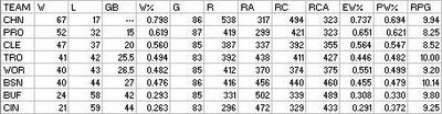
Chicago dominated the league in all three percentage categories, although their record W% was not matched in EW% or PW%. Troy managed to pull themselves up to respectability, while Buffalo went in the opposite direction. Boston fell out of the first division for the first time, and Cincinnati took the cellar in their swan song for the third time in the first five NL campaigns.

In 1880, the league hit .255/.271/.329, for a .094 SEC, 4.69 runs and 23.96 outs per game. The 4.69 runs was easily the lowest yet in the NL, as was the error rate (as seen in the .901 fielding average). Compared to 1876, R/G had dropped by 1.2 and the fielding average had improved by 35 points.

CHICAGO

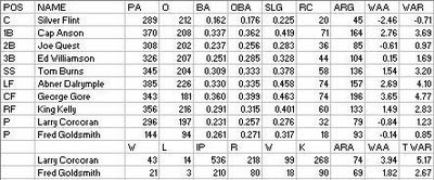
The White Stockings exploded on the league with improvement both at the plate and in the field, but it was the defense that made the big step forward. The regular lineup was largely intact (rookie Tom Burns took over shortstop, while King Kelly was pilfered from Cincinnati and took right field), so much of the credit would seemingly have to be given to the brilliant tandem of young pitchers the club unearthed. Twenty-one year old Larry Corcoran was a true rookie, while twenty-four year old Fred Goldsmith had worked 63 average innings (97 ARA) for Troy in 1879.

Offensively, Ed Williamson took a major step back in value while Silver Flint went from above average to below replacement level. This was offset, though, by a full season from a healthy Anson; replacing John Peters’ aging bat with Burns; and most of all, star-caliber seasons from Abner Dalrymple and second-year center fielder George Gore.
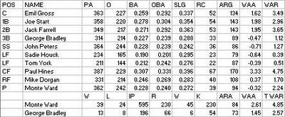
PROVIDENCE

Providence tried Mike McGeary (shipped off to Cleveland after being removed) and Monte Ward at manager before turning the reigns over to Mike Dorgan (who served in that role for the Stars in 1879). Under Dorgan, the team went 26-12 and kept pace with Chicago; of course, they were already hopelessly buried along with the rest of the league.

The Grays did not have the services of Bobby Mathews this season (I’m not sure why, and some very perfunctory searching didn’t turn anything up), but they replaced him ably with Troy’s George Bradley. The reserve clause hit the team hard, though, as George Wright decided to retire to focus on his sporting good business rather than stay on (he appeared in one game for Boston before the Grays blocked further appearance on the basis of having reserved him); Jim O’Rourke was allowed to slip back to Boston, as he was not reserved.

John Peters brought his declining offense with him from the Windy City, while Jack Farrell was salvaged from Syracuse. Sadie Houck went to Cleveland mid-season.

The catching duties were turned over to Emil Gross, who had a promising rookie campaign in 1879 (a 167 ARG in 136 PA). He caught every inning of every game, and demonstrated that his offensive showing had been no fluke.

CLEVELAND

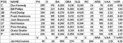
The Blues improved by twenty games largely due to the emergence of Jim McCormick as a very good (and iron; he pitched 63 innings more than anyone else in the league) pitcher, and rookie second baseman Fred Dunlap. Frank Hankinson and Orator Shaffer came over from the White Stockings while Pete Hotaling came from Cincinnati.

Rookie Ned Hanlon took over in the outfield after Al Hall, formerly with Troy, broke his league early in the season in Cincinnati. The Reds generously held a benefit on his behalf; Cleveland owner J. Ford Evans did not go, saying “I have to go to a champagne breakfast.” He then released Hall and left him stranded in the Queen City.

McCormick’s fine season was highlighted by his performance against the juggernaut White Stockings. No team (other than Cleveland) won more than three games from them the entire season. McCormick beat them four times himself. The most memorable was the July 10 game that snapped Chicago’s 21 game winning streak. Fred Dunlap cracked a two-run homer in the bottom of the ninth to give McCormick a 2-0 victory over Fred Goldsmith.

TROY

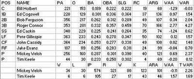
The Trojans overhauled half of their lineup, finding productive rookies in Roger Connor and Pete Gillespie, promoting John Cassidy and manager Bob Ferguson to regular roles, and bringing in Bill Holbert from Syracuse and Ed Cogswell from Boston (Cogswell took first base away from Dan Brouthers, who played in just three games). Their most fruitful move was replacing George Bradley as primary pitcher with a pair of outstanding rookies: 23 year old Tim Keefe and 20 year old Mickey Welch. Along with Chicago’s Fred Goldsmith, they made three outstanding rookie pitchers unearthed by the team.

The NL relented this season and allowed Troy to play their profitable exhibitions with neighboring Albany, but the rivalry almost cost the Trojans their spot in the league. Their May 15 game at Providence was rained out, and rescheduled for Monday the 17th (no Sunday ball in the pious NL, of course). Troy was scheduled to play Albany and chose to forfeit the league game so as not to miss the more profitable engagement. The Grays were furious and sought Troy’s expulsion, but the league decided that it was a “technical violation” since it was a make-up and not a regularly scheduled game. However, this was coupled with a strong warning not to do it again.

Boston and Providence had been so sure that Troy would get the boot that they had already started negotiating with Trojan players (the Reds with Caskin, the Grays with Cogswell, Holbert, and Welch).

Also of note is Keefe’s performance; I have him down for a 46 ARA, which is obviously great, but wouldn’t set any records. Baseball-Reference.com and other sources credit him with the best ERA+ in baseball history, 294. First, I’m not crazy about him being eligible as he only tossed 105 innings (the B-R criterion is one IP per team game; he qualifies, but pitching 105 innings in 83 team games while other pitchers in the league are pitching 500+ innings is not quite the same as 180 innings in 162 team games, as far as I’m concerned).

Secondly, Keefe allowed a large number of unearned runs, even for the time and place. He allowed 27 runs, only 10 of which were earned (37%). The team as a whole allowed 51% earned runs, while the league allowed 50% earned runs. It was certainly an impressive rookie season, but it was nowhere near being one of the greatest seasons of all-time.
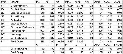
WORCESTER

The Brown Stockings had to struggle to even gain entry to the National League, which had a rule that a city must have a population of 75,000 or else require unanimous approval from the other clubs. Troy opposed the Brown Stockings’ bid because they wanted to see their rival Albany admitted. To get around this, the league expanded territory to a four mile radius around the city, bringing Worcester up to the threshold.

The team used a variety of innovative techniques for financing, including: selling shares in the club (season tickets included) for $35, selling women-only season tickets, and holding a benefit walk that attracted 3,000 people.

The Brown Stockings lineup was comprised primarily of rookies and former NLers. Rookie pitcher Lee Richmond was a Brown University product who pitched one game for the Reds in 1879; he spent the winter working with backup catcher Doc Bushong (41 games). Fellow rookie Fred Corey had pitched five games for the Grays in ’79.

Rookies Harry Stovey and Arthur Irwin were the team’s top position players, while Art Whitney and George Wood were also rookie contributors. Charlie Bennett, the fine catcher, had last played for Milwaukee in 1878, and Chub Sullivan for Cincinnati in that year. The team was filled out by George Creamer of Syracuse and Buttercup Dickerson of Cincinnati.

In the campaign against the sinful Reds, one of the leading voices was the Worcester Spy. Unfortunately for the Brown Stockings, Cincinnati was in fact expelled and replaced by Detroit. The new franchise hired away the Brown Stockings’ manager, Frank Bancroft.
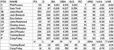
BOSTON

The Reds turned in what was easily the worst season in franchise history. The team had never before finished below a .557 W% or below third place, dating back to 1871. They also won NA/NL pennants in 1872-1875 and 1877-1878.

What was the cause? The team suffered WAR declines at every position except second base and right field (where Jim O’Rourke returned after a year in Providence). Phil Powers and Sam Trott, a pair of rookie catchers (Powers had played eight games for the White Stockings in 1878, while Trott was purchased from the independent Washington Nationals) did not match the production of Pop Snyder. Ed Cogswell was replaced at first base by John Morrill, which left a whole at third base. Ezra Sutton filled that spot, leaving a whole at short, where John Richmond, previously of Syracuse, did not play well. John O’Rourke had another fine season, but it was not as good as his rookie campaign.

However, the biggest problem was the collapse of Tommy Bond. Bond had totaled 12.4 WAR in his first three years in Boston and was the NL’s top pitcher in each of these seasons for my money. He fell to a 107 ARA; Curry Foley, the #2 pitcher, did not pitch any better than he had in 1879 (his ARA improved from 114 to 112), but he continued his fine hitting and contributed at first base and right field.

The decision to suspend and have one of their best players, Charley Jones, blacklisted did not help either. Soden ran the team along with two other men; they were collectively known as the Triumvirs and were considered very cheap. Supposedly they even collected the tickets at the gate themselves on occasion. Jones and Soden did battle when the outfielder asked for payment (reported as $378) while on a road trip. While the payday had technically come, it was customary for players to be paid when the team returned home. Soden decided to leave Jones behind in Cleveland and claimed he had jumped the club. Jones then took the matter to an Ohio court and got a ruling in his favor; this was enforced by taking a share of the receipts when the Reds played in Cleveland. Jones used this money to buy a laundry.

As an aside, a lot of these anecdotes may be apocryphal, to some extent or another. I am not a historian, and I have relied solely on secondary sources to gather them. So take them with a grain of salt, and please don’t get the impression that I’m trying to pass this off as a meticulous, 100% accurate history, or that I’m trying to pass myself off as a historian.

Case in point is how I have switched to using “Reds” as a nickname for Boston in this entry. Richard Hershberger pointed out in the comments that “Red Caps” was never used by primary sources, and he believes that the confusion stems from a St. Paul club listed as the Red Caps, which has bled over into the Boston NL franchise because of some writer’s misunderstanding. He suggested using “Bostons”, as this was the most commonly applied name, more so than even “Boston”. I did not go that far, but I do not want to contribute any further to the proliferation of Red Caps.

As long as somebody, somewhere referred to the team by a given nickname, that’s enough for me. I treat it as if I was writing about contemporary baseball, in which case I might refer to the “Bronx Bombers”, “the Tribe”, “the White Elephants”, “the Buccos”, etc. Using those nicknames in those veins is in no way a claim that they are official, team-approved, used extensively in press coverage, etc. It is in that same spirit that I used nicknames for the nineteenth century clubs.

BUFFALO

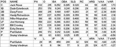
The Bisons collapsed from third place to seventh place and a sub-.300 W%. It didn’t help that Pud Galvin’s innings declined from 593 to 459, with his effectiveness also taking a serious hit (95 ARA to 113); he also held out in San Francisco very early in the season. Rookie #2 pitcher Stump Wiedman, just nineteen, was bad in the box and atrocious at the plate. Oscar Walker, decent at first base in 1879, was fined $50 in early June for breaking a temperance pledge and fell out of favor, playing in just 34 games.

Chuck Fulmer, my choice for all-star second baseman in 1879, played in just eleven games. The team also lost catcher and manager John Clapp. Rookie catcher Jack Rowe was solid, and rookie shortstop Mike Moynahan was very good in limited time (106 PA), but fellow rookies Dude Esterbrook and Ecky Stearns combined for sub-replacement level performance.

CINCINNATI

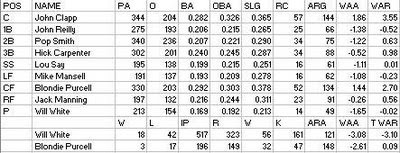
This Reds club was not the same one that competed in the NL in 1879. Instead, an independent team called the Stars was drafted to replace them. Thus, these new Reds did not have many carryovers from the decent 1879 club. The White brothers were the only returnees amongst the regulars, and Deacon missed much of the first half tending to his ailing wife, playing right field when he returned. Will suffered through a terrible season (-3.1 WAR). John Clapp was brought in from Buffalo to manage and catch; Hick Carpenter, Mike Mansell, and Blondie Purcell were all salvaged from Syracuse; and Jack Manning had last played with the Reds in 1878. Rookies Long John Reilly, Pop Smith, and Lou Say contributed little.

Any disappointment Reilly may have had over a replacement-level rookie season was probably offset by sheer joy of being alive. According to his SABR BioProject entry (written by David Ball, whose “Nineteenth Century Transactions Register” has also been a valuable source), Reilly and the Reds played in Providence on June 10, then had a couple of off days. So he went to New York City on a Long Island Sound steamer. On the June 11 return voyage, his boat, the Narragansett collided with another boat, the Stonington.

Reilly helped in various rescue efforts on board, then jumped into the water when it seemed the ship would sink and floated for around an hour while holding to piece of wood before being rescued. The Reds and Grays played again the next day, unsure of whether Reilly was dead or alive at first. He returned to the lineup on the 15th.

While errors were still quite common, the Reds’ August 28 game against Troy was a little excessive: nine errors in the fourth inning and sixteen in the game, which they lost 13-2.

The Reds as a major league franchise would not share the same joy of being alive as their first baseman once the season was over. The team insisted on renting its park out to non-league clubs that sold alcohol and played on Sundays. This led to calls for punishment against the sinners, with the aforementioned Worcester Spy a major player. A Cincinnati backer fired back against the critics, “Puritanical Worcester is not liberal Cincinnati by a jugful. We drink beer…as freely as you used to drink milk” (Seymour, pg. 92). Additionally, Cincinnati refused to accept Worcester’s chosen umpire, Foghorn Bradley, in retaliation (at this time, umpires were chosen by and would travel with the visitors).

On October 6, the NL voted unofficially to ban alcohol sales and Sunday ball on team grounds, 7-1. Cincinnati refused to sign a pledge to obey the rule, and was then expelled for not promising to vote yes when the matter came up for a formal vote.

(The league leaders and my "all-star" picks will be a seperate post, as Blogger will not allow to write anything past this point without double spaces. Why? I don't have a clue, and I'm not going to learn HTML to divine it. Also notice the single spaces after periods, which were double spaces in my Word document.)

Monday, July 14, 2008

Run Estimation Stuff, pt. 4

In this installment, I will look at the accuracy of the formulas we have created compared to the accuracy of some other run estimators. Let me pile on some caveats here:

1. I am certainly not claiming that accuracy in terms of RMSE on actual major league teams is the only standard by which to evaluate a run estimator, or even the most important. It is something interesting to look at.

2. The data used for the test is 1990-2005, except 1994. This overlaps with the sample data we used to derive our formulas, giving them an inherent advantage. This should be considered when looking at the results.

3. A corollary to #1, it must always be remembered that there is correlation between the various offensive events. A category like SF, which guarantees that a run has been scored, can be treated in a way such that it increases the accuracy of a formula, but decreases its accuracy in application to players and in theory. It has always been a source of amusement for me that there is somewhat of an overlap between the crowd that claims run estimators are subject to the ecological fallacy and the crowd that exalts lowest RMSE above all other virtues.

First, I will compare a group of estimators that only use the basic statistics (AB, H, D, T, HR, W, SB, and CS). This includes Bill James’ Stolen Base RC (RC), Jim Furtado’s Extrapolated Runs Basic (XR) , a variant of Paul Johnson’s ERP (ERP), the basic LW introduced in the first part of this series from Ruane’s data (LW-R), the older BsR version that I have used (Old BsR), the two BsR versions introduced in the second installment (B1 and B2), the two simple BsR versions from David Smyth introduced in the last installment (sBsR1 and sBsR2; remember that these do not use SB or CS) and two regression equations (Reg1 and 2, formulas at the bottom of the post).

I have included two measures of accuracy: RMSE and average percentage error ABS(R-RC)/R:


I’m a little disappointed that the new BsR formulas came out worse than the old one, but I’m not sure what data I calibrated that one on. Of course, the new versions benefited at least a bit from this phenomenon too. Again, to really do a fair test, you would have to test on data outside of the sample used to create the formula. I should do that, but I have done those kinds of tests before. My goal here is not to show which estimator is the “best”, even within the sphere of RMSE analysis.

It is also true, as David Smyth pointed out in a discussion on The Book Blog, that the weights which return the “correct” linear weights values are not necessarily those that will be most accurate for estimating team runs for normal teams. This could be even more of a factor when the linear weights themselves have been adjusted to equal total runs scored, as they have not accounted for all of the possible outcomes (for example, Ruane’s linear weights ignore reached on error, wild pitches, and several other events). This is why I in no ways intend the formula here to supercede Tango Tiger’s full Base Runs equation and corresponding linear weights. These are simply BsR versions that utilize the full complement of official statistics while considering nothing beyond those.

The regression equations come in front, which they should, considering that they are specifically tailored to work with the 430 unique batting lines in this sample. The formulas for them are in the bottom section and I’ll repeat myself again on regression there.

With that aside, let’s move on to looking at estimators that take advantage of all of the official offensive categories. Here, we have ERP again; Bill James’ Tech-1 RC, HDG-24 RC, and revised RC; another old BsR version of mine; LW-R, the weights we derived in part one from Ruane’s study; “RC match”, which is RC with B weights to match the target weights; “CR match”, which is loosely based on Eric Van’s Contextual Runs framework and also matches the target weights; and the Full-1 through 4 BsR versions introduced in part two (plus the F-1 version with a corrected walk coefficient):

Again, the regression equations win out as they should. My older BsR version does better than the new ones, which makes me suspect that I calibrated it on a dataset that heavily overlapped this one. While I introduced four new BsR equations here, they were all almost exactly the same when applied to these real teams. The “winner”, Full-2, is one based on initial baserunners and all outs, for what it’s worth, which is not a lot. The choice of which version to use should be based on how they would do theoretically and how their weights stack up rather than which had a RMSE .02 lower than the others.

One thing to note is that James’ Tech-1 RC formula is not particularly accurate, at all, at least for recent years. Stolen Base RC, despite ignoring IW, SH, SF, DP, and HB, has a RMSE nearly three runs lower than Tech-1. James himself does not use Tech-1 anymore; he supplanted it first with the HDG-24 formula and than with the one he uses now that doesn’t have a catchy name. However, some folks out there still use Tech-1, and even if you are not concerned about all of the issues that have been raised about the RC model itself, you should recognize that Tech-1 is a poor estimator.

Since we have Ruane’s empirical weights, it would be interesting to compare the BsR-generated weights for various seasons. I did not do a comprehensive analysis, but I did take a look at two extreme leagues (the 1968 NL and the 1996 AL; of course, “extreme” on the league level is nothing like extreme on the team or, to an even greater degree, the player level). Again, this is not in anyway intended to be a conclusive study, it is just an interesting platform to use for further discussion. I used the Full-1 version of BsR (initial baserunners, batting outs) to generate the BsR values:

1968 NL:

1996 AL:

The BsR intrinsic weights are within .03 runs for each event except the triple in 1968 and the sac fly in both seasons. Perhaps the high B weight for the triple keeps the coefficient artificially high even in low run environments. In the case of the sac fly, Base Runs weights it nearly equally in 1968 and in 1996. Apparently, my treatment of the event does not allow its value to fluctuate as much as it actually does. Perhaps treating it as a removed baserunner would do the trick, although if you do that you pretty much have to count it as a guaranteed run to balance things out, and I don’t like the implications of that. If I had my druthers, the official stats would give us breakdowns for flyouts and groundouts instead of the subcategories of SF and DP, and then this wouldn’t be an issue at all.

Miscellaneous Formulas

Full ERP = (TB + .792H + W + HB - .5IW + .3SH + .7(SF + SB - DP) - CS - .292AB - .031K)*.322

This is one I had sitting around from years ago; it obviously does not properly value the events, but that’s part of the reason why I included it--its accuracy with real teams is not that far off from the others, despite having some obvious flaws. Let it serve as another example about the limitations of RMSE.

Reg-1 = .222H + .302TB + .336W + .242SB - .177CS - .113(AB - H)

Reg-2 = .553S + .705D + 1.117T + 1.499HR + .330W + .240SB - .215CS - .113(AB - H)

Reg-3 = .225H + .290TB + .366W - .336IW + .267HB + .151SB - .121CS + .640SF + .001SH - .100(AB - H) - .020K - .379DP

Reg-4 = .552S + .645D + .993T + 1.458HR + .353W - .287IW + .346HB + .144SB - .141CS + .715SF - .026SH - .101(AB - H - K - DP) - .117K - .475DP

Take a look at how the third and fourth formulas treat the double. The formula that considers the hit types separately weight the double at .65 runs, while the version that uses hits and total bases weight it at .81 runs. The dataset used was exactly the same; the only difference is the variables that were fed into the regression. We would expect to have a slight discrepancy between the value of an extra base hit from the approach of valuing each extra base equally. But a .16 run gap? Some of it is the product of adding the sacrifice fly, some of it is just the fact that the inputs are different and the mathematical procedure does not know anything about baseball. The fact that such a difference can occur for the same dataset should illustrate to anyone who still places a large amount of faith in regression equations for the job of estimating event values that it may be a misguided faith.

If you are concerned about the ecological fallacy, regressions are the methods that you should worry about. The best example is the sacrifice fly. From Ruane’s data, it is apparent that at the average scoring level of 1960-2004, the sacrifice fly is a neutral play from a run expectancy standpoint (-.01 runs). When that value is converted to absolute runs, it is worth about +.15 runs.

However, regression procedures know nothing about baseball reality. They only know about the combinations of numbers you give them, and the correlation between the variables. Sacrifice flies correlate decently with runs scored (better than triples, hit batters, or steals in this sample), and each sac fly is a guaranteed run for the team. You can see that the sac fly is evaluated as being worth more than a double, which is absurd on its face.The double is also only .1 runs more valuable than a single in the regression equation.

"Old" BsR Formulas:

A = H + W - HR - CS

B = (2TB - H - 4HR + .05W + 1.5SB)*.76

C = AB - H

A = H + W - HR + HB - CS - DP

B = .781S + 2.61D + 4.28T + 2.42HR + .034(W - IW + HB) - .741IW + 1.29SB + .125CS + 1.07SH + 1.81SF + .69DP - .029(AB - H) - .086K

C = AB - H + SH + SF

Monday, July 07, 2008

Run Estimation Stuff, pt. 3

Base Runs and Runs Created have many similarities that are easily apparent. Each has an A factor that represents baserunners and a B factor that represents advancement. Each has a C factor that in some way reflects what Bill James called “opportunity”, but James used plate appearances while Smyth uses outs.

The two fundamental differences between the models are 1) their treatment of the home run and 2) how they estimate score rate (the proportion of baserunners that score). BsR recognizes that a home run always results in at least one run, and thus splits them off into a D factor. This modification not only credits each homer with creating at least one run, but it alters the BsR A factor. Since the run scored by the batter who hits the longball has already been accounted for, home runs are removed from baserunners.

Then, since BsR estimates score rate as a proportion (B/(B + C)) rather than as a ratio (B/C), it adheres to the obvious constraint that “runs scored by baserunners <= baserunners”, which RC does not adhere to. If B>C, than RC predicts that more runs will score than their were runners on base.

This is not to say that BsR is a perfect model, because of course it is not. For example, BsR does not adhere to the rule that you can leave a maximum of three on base per inning. In some extreme situations it could return a negative run estimate (although the simple versions that do not subtract anything from the B factor have a lower bound of zero). But these things are also true of Runs Created.

Another flaw of BsR is that in some extreme cases, the intrinsic weight of a triple is greater than that of a home run. This is obviously absurd, although Tango Tiger has developed a workaround for this situation. However, while RC does not have that flaw, it is not necessarily a point in RC’s favor. It’s better to have the triple be weighted higher than a homer, but both weighted somewhat in the vicinity of their actual value than to have both wildly overvalued. That is not to say the triple problem is a good thing for BsR; it’s a clear shortcoming. It just doesn’t hurt its standing against RC, as any time BsR says that a triple is worth more runs than a home run, RC will be telling you that they are both are much more valuable than they actually are.

The only claim here is that BsR is a better model than RC, in almost all regards. You might be able to find an extreme situation that a particular RC version will handle better than a particular BsR version, but the vast majority of cases go to BsR and the logic of the model is a clear advantage for BsR. There is also no fundamental rule of baseball (such as the maximum three runners stranded per inning) that RC adheres to when BsR does not, at least not that I am aware of. Base Runs is the best simple, dynamic model for run scoring that we have. Of course, I grant that simulations and Markov models can be superior if designed properly. However, those take massive spreadsheets or stand-alone programs to implement. As far as formulas that can be implemented quickly on a spreadsheet (and explained in English to those unfamiliar with linear algebra or computer programming) go, Base Runs is the best model.

Anyway, what I want to do here is to examine RC and BsR head-to-head in the manner that Tango suggested here. First, let’s look at Bill James’ latest RC version, remembering that RC is always A*B/C:

A = H + W + HB - DP - CS
B = 1.125S + 1.69D + 3.02T + 3.73HR + .29(W - IW + HB) + .492(SB + SH + SF) - .04K
C = AB + W + HB + SH + SF

As will be demonstrated in the next segment, this formula is more accurate than any of the BsR versions we came up with when used on the 1990-2005 team data. I don’t put a lot of stock in this, but I feel obliged to mention it in the interests of full disclosure (lest I be accused of being a BsR “fanboy” as I have been in the past, by one of the idiots who posts at a certain site that sometimes links to stuff like this, although thankfully not as much as they did in the past).

Let’s take a look at the intrinsic weights generated by this formula for the 1960-2004 period, compared to the target weights from Ruane’s research:


I will let that stand without comment; if the arguments of others as well as my own feeble efforts have not yet convinced you of the importance of approximating empirical linear weight values, nothing I can say here will help. If you hold that view, this table should be very revealing with respect to the Runs Created model, or at the very least the manifestation of it that is currently in use.

Just as we did for BsR, we can find the B coefficients for RC necessary to match our target linear weights. They are:

B = .634S + 1.640D + 2.594T + 3.844HR + .105(W - IW) - .337IW + .189HB + .652SB + .416CS + .157(AB - H - K - DP) + .025K + .146DP + .629SH + .911SF

You can see that these weights are superficially similar to the BsR B weights; of course the home run is a big exception, and there certainly are some discrepancies, but they are in the same ballpark.

We can also “dumb down” Base Runs in order to compare it to the Runs Created model. David Smyth has recently suggested this type of approach as the most basic Base Runs model. What we will do is not give the home run the special treatment of being split off from baserunners and always credited with creating at least one run.

This is not to say that the home run should not be treated as BsR does. The home run, as opposed to other (or possible) categories that always indicate a run scored, like the sacrifice fly, is unique not as a scoring category but as an event defined by the rules of the game. A sacrifice fly, or a RBI groundout, is just an accounting category--it's a way of more specifically describing the outcome of a given event that could have also been classified an out, a groundout, etc. The home run is not just an accounting category; it is an event set aside in the rules of baseball that entitles the batter and any runner to score automatically without the threat of being put out. While there are other events that allow one to score without risk (a bases loaded walk, for instance), the home run is the only event that can do so independently of what precedes or follows it in an inning.

That digression aside, a simple version of BsR suggested by Smyth is:
A = H + W
B = (2*TB - H + HR)*.75
C = AB - H
BsR = A*B/(B + C)

Another version he offered is B = (2*TB - H)*.79.

We could optimize this equation to match target linear weights in the same way that we did in the previous installment, but that would be overkill. It defeats the point of a “simple” formula to include small fractional weights for walks and outs in the B factor.

The second version in particular does a decent job of estimating linear weight values: .52, .83, 1.14, 1.45, .36, -.11 for 1960-2004 (S, D, T, HR, W, O). To me, this in an illustration of the fact that BsR is a step forward over RC in its approach to estimating score rate, without even considering its treatment of the home run.

We have looked at how we can move RC closer to BsR by switching to a proportional estimate of score rate. We could also move RC closer to BsR by retaining a ratio estimate of score rate, but instead dealing with the home runs specially. This would give us a model along the lines of Runs = A*B/C + D.

In fact, this is a construct that has been used for a run estimator, namely Eric Van’s Contextual Runs. Here we will make a generic version to would match our target linear weights:

A = H + W - HR + HB
B = .349S + 1.018D + 1.652T + .915HR - .004(W - IW) - .297IW + .053HB + .434SB - .598CS + .153(AB - H - K - DP) + .065K - .730DP + .467SH + .654SF
C = AB - H + SH + SF

Van uses an initial baserunner, full out construct, but I just want to illustrate how the coefficients directly compare to the RC and BsR versions here. Obviously I am not attempting to supersede his definition of his own estimator; consider this a generic, nameless A*B/C + D model. However, it would be disingenuous to present such a model without acknowledging Van's work.

The bottom line is that all of these models are inferior to the full Base Runs model of A*B/(B + C) + D. Is it possible that someone could develop a better estimator of score rate? Sure, it’s possible. However, it won’t be easy to find, and it is almost certain that it would be a lot more complex than B/(B + C).

When you look at the measures to which Bill James has resorted to prop up the accuracy of RC, you have to ask why not just take one more step and take HR out of A? That is the only difference between the two formulas at this point, once James abandoned using TB in the B factor (instead considering S, D, T, and HR separately) and went to two decimal place weights.

The claim that RC is more simple than BsR, computationally, is now hinging just a few additional mathematical operations (subtracting HR from A, adding them in D, adding B and C, and depending on which BsR version you use, adding and multiplying by a coefficient for a few miscellaneous events in B). If it is really simplicity that you crave, a simple linear weights formula can’t be beat. If you are willing to put up with the “complexity” of Runs Created, it seems very odd to me that you would find Base Runs to be a bridge too far.

I do not really care if Bill James wants to continue to use RC; after all, he developed it, and it has influenced the superior estimators that followed. I imagine that it’s hard to let go of your own creation that was once considered the gold standard (I wouldn’t know because I am no Bill James, not by a longshot, and have never been in that position). What I fail to understand, though, is why anyone else continues to use Runs Created (other than its most simple incarnations for quick and dirty estimates in the same vein as OPS and its cousins).