Enby Distribution, pt. 11--Game Expected W%

This is (finally!) the last post in this series, at least for now.

In the Mets essay for the 1986 Baseball Abstract, Bill James focused on data he was sent by a man named Jeffrey Eby on the frequency of teams scoring and allowing X runs in a game, and their winning percentage when doing so. After some discussion of this data, and a comparison of the Mets and Dodgers offense (the latter was much efficient at clustering its runs scored in games to produce wins), he wrote:

“One way to formalize this approach would be to add up the ‘win expectations’ for each game. That is, since teams which score one run will win 14.0% of the time, then for any game in which a team scores exactly one run, we can consider them to have an ‘offensive winning percentage’ for that game of .140. For any game in which the team scores give runs, they have an offensive winning percentage of .695. Their offensive winning percentage for the season is the average of their offensive wining [sic] percentages for all the games.”

It stuck James at the time, and me reading it many years later, as a very good way to boil the data we have about team runs scored by game and boil it down into a single number that gets to the heart of the matter – how efficient was a team at clustering their runs to maximize their expected wins? James (in the essay) and I (for the last eight seasons or so on this blog) used the empirical data on the average winning percentage of teams when scoring or allowing X runs to calculate the winning percentage he described. I have called these gOW% and gDW%, for “game” offensive and defensive W%. However, there are a number of drawbacks to using empirical data.

To repeat myself from my 2016 review of the data, these include:

1. The empirical distribution is subject to sample size fluctuations. In 2016, all 58 times that a team scored twelve runs in a game, they won; meanwhile, teams that scored thirteen runs were 46-1. Does that mean that scoring 12 runs is preferable to scoring 13 runs? Of course not--it's a quirk in the data. Additionally, the marginal values (i.e. the change in winning percentage from scoring X runs to X+1 runs) don’t necessary make sense even in cases where W% increases from one runs scored level to another.

2. Using the empirical distribution forces one to use integer values for runs scored per game. Obviously the number of runs a team scores in a game is restricted to integer values, but not allowing theoretical fractional runs makes it very difficult to apply any sort of park adjustment to the team frequency of runs scored.

3. Related to #2 (really its root cause, although the park issue is important enough from the standpoint of using the results to evaluate teams that I wanted to single it out), when using the empirical data there is always a tradeoff that must be made between increasing the sample size and losing context. One could use multiple years of data to generate a smoother curve of marginal win probabilities, but in doing so one would lose centering at the season’s actual run scoring rate. On the other hand, one could split the data into AL and NL and more closely match context, but you would lose sample size and introduce more quirks into the data.

Given these constraints, I have always promised to use Enby to develop estimated rather than empirical probabilities of winning a game when scoring X runs, given some fixed average runs allowed per game (or the complement from the defensive perspective). Suppose that the major league average is 4.5 runs/game. Given this, we can use Enby to estimate the probability of scoring X runs in a game (since the goal here is to estimate W%, I am using Enby with a Tango Distribution c parameter = .852, which is used for head-to-head matchups):



From here, the logic to estimate the probability of winning is fairly straightforward. If you score zero runs, you always lose. If you score one run, you win if you allow zero runs. If you allow one run, then the game goes to extra innings (I’m assuming that Enby represents per nine inning run distributions, just as we did for the Cigol estimates. Since the major league average innings/game is pretty close to nine, this is a reasonable if slightly imprecise assumption), in which case we’ll assume you have a 50% chance to win (we’re not building any assumptions about team quality in as we do in Cigol, necessitating an estimate of winning in extra innings that reflects expected runs and expected runs allowed). So a team that scores 1 run should win 5.39% + 10.11%/2 = 10.44% of those games.

If you score two runs, you win all of the games where you allow zero or one, and half of the games where you allow 2, so 5.39% + 10.11% + 13.53%/2 = 22.26%. This can be very easily generalized:

P(win given scoring X runs) = sum (from n = 0 to n = x - 1) of P(n) + P(x)/2

Where P(y) = probability of allowing y runs

Thus we get this chart:



It should be evident that the probability of winning when allowing X runs is the complement of the probability of winning when scoring X runs, although this could also be calculated directly from the estimated run distribution.

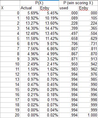
Now, instead of using the empirical data for any given league/season to calculate gOW%, we can use Enby to generate the expected W%s, eliminating the sample size concerns and enabling us to customize the run environment under consideration. I did just that for the 2016 majors, where the average was 4.479 R/G (Enby distribution parameters are r = 4.082, B = 1.1052, z = .0545):



The first two columns compare the actual 2016 run distribution to Enby. The next set compares the empirical probability of winning when scoring X runs (I modified it to use a uniform value for games in which 12+ runs were scored, for the purpose of calculating gOW% and gDW%) to the Enby estimated probability. The Enby probabilities are generally consistent with the observed probabilities for 2016, but as expected there are some differences, and note that Enby is assuming independence of runs scored and runs allowed in a single game which environmental conditions alone make an assumption that can be most positively described as “simplifying”.

The resulting gOW% and gDW% from using the Enby estimated probabilities:



There is not a huge difference between these and the empirical figures. One thing that is lost by switching to theoretical values is that the league does not necessarily balance to .500. In 2016 the average gOW% was .497 and the average gDW% was .502.

However, the real value of this approach is that we no longer are forced to pretend that runs are equally valuable in every context. Note that Colorado had the second-highest OW% and third-lowest DW% in the majors. Anyone reading this blog knows that this is mostly a park illusion. If you look at park-adjusted R/G and RA/G, Colorado ranked seventeenth and nineteenth-best respectively, with 4.42 and 4.50 (again the league average R/G was 4.48), so the Rockies were slightly below average offensively and defensively. While we certainly don’t expect our estimate of their offensive or defensive quality using aggregate season runs to precisely match our estimate when considering their run distributions on a game basis (if they did, this whole exercise would be a complete waste of time), it would be quite something if a single team managed to be wildly efficient on offense and wildly inefficient on defense.

When we consider that Colorado’s park factor was 1.18, in order to compute gOW%/gDW% in the run environment in which they played, we need to take the league average of 4.479 R/G x 1.18 = 5.29. (We could of course use the NL average R/G here as well; I’m intending this post as an example of how to do the calculations, not a full implementation of the metrics. For the same reason, I will round that park adjusted average up a tick to 5.3 R/G, since I already have the Enby distribution parameters handy at increments of .05 R/G). With c = .852, we have an Enby distribution with r = 5.673, B = .9363, z = .0257. The resulting Enby estimates of scoring frequency and W% scoring/allowing X runs are:



Using these estimated W%s, the Rockies gOW% drops from .560 to .485 and their gDW% increases from .437 to .508. As suggested by their park-adjusted R/G figures, Colorado’s offense and defense were both about average; their defense fares a little better when looking at the game distribution than when using aggregate totals, and the opposite for the offense.

Some readers are doubtlessly thinking that by aggregating at the season level, we’ve lost some key detail. We could have looked at Colorado home and road games separately, each with a distinct set of Enby parameters and corresponding probabilities of winning when scoring X runs rather than lumping it altogether and applying the park factor that considers that half of the games are on the road. This of course is true; you can slice and dice however you’d like. I find the team seasonal level to be a reasonable compromise.

This is beyond the scope of this series, so I will mention it briefly and move on. I have previously combined gOW% and gDW% into a single W% estimate by converting each into an equivalent run ratio using Pythagenpat math, then using Pythagenpat to convert those ratios into a W% estimate. This makes theoretical sense, although it loses sight of using the actual runs scored and allowed distributions of a team in a season and rearranging them (“bootstrapping” if you must). It occurred to me in writing this post that I could just use the same logic I use to convert Enby probabilities of scoring X runs into an estimated W% for the team. For example, we could use the Rockies runs scored distribution to estimate how often they would win when allowing x runs and use this in conjunction with their runs allowed distribution to estimate a W% given their runs allowed distribution. Then we could do the same with their runs scored/runs allowed to estimate a W% given their runs scored distribution. Averaging these two estimates would, in essence, put together every possible combination of their actual runs distribution from the season and calculate the average expected wins. For a simple example that avoids “ties”, if a team played two games, winning one 3-1 and the other 7-5, we would make every possible combination (3-1, 3-5, 7-1, 7-5) and estimate a .750 gEW%, compared to a 1.000 W% and a .720 Pythagenpat W%.

Here’s an example for the 2016 Rockies:



The first two columns tell us that the Rockies scored two runs in 16 games and allowed two in 15 games. After converting these to frequencies, we can easily calculate the probability of winning giving that the team scores X runs in the same manner as we did above with Enby probabilities. For example, when the Rockies score two runs, they will win if they allowed zero (5.56%) or one (8.64%), and half of games in which they allow two (9.26%), for a win probability of 5.56% + 8.64% + 9.26%/2 = 18.8%. Figured this way, the Colorado’s gOW% is .494, their gDW% is .496, and thus their gEW% is .495. Please note that I’m not suggesting that using the team’s actual frequencies of scoring/allowing X runs is preferable to using league averages or Enby. Furthermore, the gOW% and gDW% components are not useful, since they make the estimate of the quality of the offense or defense dependent on its counterpart.