Akousmatikoi Win Estimators, pt. 4: Best Fits and Accuracy

Herein I’ll be using the expansion era (1961 – 2019) data for all major league teams to calculate the RMSE of the various Akousmatikoi win estimators we’ve discussed. This exercise is not intended to prove which metric is “better” or “more accurate” than the others, but rather is intended to give you a feel for the differences between the various approaches when used for major league teams. What I am calling the Akousmatikoi family of win estimators is built on the conceit that Pythagenpat is the “best” win estimator, and uses it as a jumping-off point to develop alternate/simplified methods that can be tied back to the parent method. As such, the contention here would be that if you want the “best” answer, you should use Pythagenpat. But if you are just looking at the standings and can apply something quick like the Kross method or 9.56 runs per win, how far off will you be for a normal team?

This is also not a “fair” accuracy test, in that we would develop the equation based on one set of data and test it on another; all of the approaches will be calibrated and tested on the 1961 – 2019 data. This will not favor one approach or another as they all will have the benefit of the same data set. I will also be including the best fits for a few of the approaches, which I think is interesting because in several cases I’ve developed the alternate to Pythagenpat shown in this series by taking the tangent line at the point where R = RA and applying it broadly. While this should work well enough as our real teams will be centered around this point, in some cases the best fit may be a little different, which might be interesting. In those cases I would probably recommend using the best fit, since the point of any of the simpler methods would be to use with real teams; there’s no need to get hung up on theoretical centering at .500.

If this is not a “fair” accuracy test, then what exactly is the point? The point is to provide information that can be us used to inform the decision of which shortcut to Pythagenpat you choose to use. There is no right or wrong answer. For example, the Kross formulas are about as simple as it gets. Are they accurate enough as a win estimator to use for quick and dirty estimates? That depends on how dirty you’d like it to be (i.e. your own determination of what level of error is acceptable), and about your own tradeoff between simplicity and accuracy.

In another sense, though, it is a fair test, because each method is operating under the same constraints (although some will benefit from having best fits determined directly while others won’t operate under that luxury). In deciding which model to use, it does make sense to have a final check when all are calibrated on all of the available data.

I will not only calculate the RMSE of the estimates compared to W%, I will also show it compared to Pythagenpat. This is not meant to imply that Pythagenpat is correct and any deviation from it is wrong, but since the presentation in this series has relied on each method’s own relationship to Pythagenpat, I think it’s of interest to identify which approaches do the best job of approximating Pythagenpat. And if you do choose to start with Pythagenpat as your win estimator of choice when attempting to be as accurate as possible, it might follow that one of the criteria you’d consider when deciding which quicker method to use is how well it tracks Pythagenpat.

I will divide the methods to be tested as follows:

Pythagorean

These will all take the form W% = R^x/(R^x + RA^x).

Pyth1: this will be Pythagenpat, where x = RPG^.282 (best-fit)

Pyth2: Fixed exponent Pythagorean where x = 2

Pyth3: Fixed exponent Pythagorean where x = 1.847 (best-fit)

Port: Davenport/Woolner’s Pythagenport, where x = 1.5*log(RPG) + .45

Cig1: formula I derived from Cigol, where x = 1.03841*RPG^.265 + .00114*RD^2

Cig2: formula I derived from Cigol to follow the Pythagenpat form, where z = .27348 + .00025*RPG + .00020*(R - RA)^2

Ratio-Based

Kross: these are the nifty equations developed by Bill Kross; when R > RA, W% = 1 – RA/(2*R); when R <= RA, W% = R/(2*RA)

Ratio: this is the general case that resolves to Kross’ equation when x = 2, although it’s not really the general-case at all since I’m using the Pythagorean best-fit of x = a = 1.847 to get these equations:

when RR > = 1, (a*RR – a + 1)/(a*RR – a + 2) = (1.847*RR - .847)/(1.847*RR + .153)

when RR < 1, 1/(a/RR – a + 1)/(1/(a/RR – a + 1) + 1) = 1/(1.847/RR - .847)/(1/(1.847/RR - .847) + 1)

Differential-Based

FixRPW: if you force an equation of the form W% = ((R-RA)/G)/RPW + .5, the best fit is when RPW = 9.71, which is equivalent to .103*((R – RA)/G) + .5

PythRPW: RPW = 2*RPG^.718, the Pythagenpat result

LinRPW: RPW = .777*RPG + 2.694, the tangent line to the Pythagenpat RPW at the average RPG/RPW for the period

BVL: W% = .9125*(R – RA)/(R + RA) + .5; the form proposed by Ben Vollmayr-Lee, although I’m using the best fit for this dataset and also rounding the intercept to .5 (it actually comes out to .49978)

BVLPyth: W% = .923*(R – RA)/(R + RA) + .5; the same equation, but using the Pythagorean best-fit exponent rather than the empirical best-fit

The RMSE shown here is actually the overall RMSE of the W% estimate, scaled to 162 games. So for each team the error is (W% - estimator)^2; the final value shown is 162*sqrt(average error):

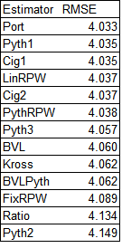
Pythagenport has a slight lead over Pythagenpat, and they are followed very closely by the estimates based on Cigol and runs per win formulations that take RPG into consideration. In the Akousmatikoi family, that is the accuacy seperator (such that it is; the overall range of RMSE values is narrow) – considering the specific run environment for the team either through a Pythagorean approach (as in the case of Pythagenport, Pythagenpat, and their Cigol knockoffs), or a two operation (multiplication and addition) or power RPW function (as in the case of LinRPW and PythRPW). The next little cluster of RMSE includes a fixed Pythagorean exponent less than 2, the BenV-L formulas (which take the team’s RPG into account but only with a simple multiplicative function, not a y = mx + b form), and the intrepid Kross formulas. A fixed RPW linear approach is next, and then surpisingly, the Kross formuals actually outperform their antecedent (in the Akousmatikoi conceit, not reality) standard Pythagorean and “Ratio”, which uses a non-2 Pythagorean exponent.

This finding is surprising, and suggests that the Ratio approach should be discarded, as it’s arguably the most complicated to calculate of all the options we’ve looked at (despite being, at least from one perspective, a mathematical “simplification” of the Pythagorean relationship). But why does it perform worse than the Kross method, which ties to x = 2, while the ratio approach ties to x = 1.847, which has a lower RMSE than using x = 2?

To answer that question, I started by looking at the most extreme teams in terms of run ratio in the period, and found what I consider to be a satisfactory answer. The team with the highest run ratio in the expansion era is the 1969 Orioles (779/517 = 1.51). Incidentally, they do not have the highest Pythagenpat W% in the era, a distinction that goes to the 2001 Mariners by a hair’s breadth over the 1998 Yankees; those teams had run ratios of 1.48 and 1.47 respectively, but they had RPGs 20% and 25% higher respectively, which made their run ratios convert to higher win ratios.

The Orioles EW% using a fixed Pythagorean exponent of 1.847 is .681. This is the calculation that “Ratio” is supposed to flatten, but it predicts a W% of just .659. I think that since this formula is developed by differentiating win ratio, and then using the estimated win ratio to calculate an estimated W%,,the linear approximation does poorly. Win ratios have a much wider range than winning percentages; if we consider .300 - .700 a reasonably range for the expected (as oposed to actual) W%s of major league teams, this is a win ratio range of .429 to 2.333. Drawing the tangent line for the point where RR = WR = 1 leaves a lot of room outside of this range where teams will fall.

The Kross formula performs better because even though (in the Akousmatikoi sense) it starts from a less accurate proposition that x = 2, it will produce a wider range of win ratio estimates. The Kross estimated win ratio for a team with a run ratio of 1.51 is 2*1.51 – 1 = 2.02, while the other approach estimates 1.847*1.51 - .847 = 1.94.

The other RMSE comparison I want to make is to Pythagenpat. Again, I am not trying to say that Pythagenpat is the standard by which all win estimators should be judged. However, it (or something similar like Pythagenport) is the most accurate version of the Pythagorean relationship that has yet been published, and since this series is an examination of alternative win estimators mathematically related to Pythagorean methods, I think it is worthwhile to see which of these alternatives hew most closely to the starting point:

The fact that the lowest RMSE is for the first Cigol estimate tells us only what we can see by observing it – that it is essentially the same formula with added terms to attempt (perhaps in vain) to increase accuracy at the extremes (this formula sets the Pythagenpat exponent to .27348 + .00025*RPG + .00020*(R - RA)^2 rather than .282). That next in line are two more close cousins, Pythagenport and the other Cigol estimate, is comforting but also uninteresting.

You’ll notice that the ranking of estimators in terms of agreement with Pythagenpat closely resembles their ranking in accuracy predicting W%, so the first grouping of methods that most closely track Pythagenpat while actually being simpler to compute are the two RPW estimates that use a “complex” function – either the power relationship or the y = mx + b form.

The next cluster is an optimized fixed Pythagorean exponent and the Ben V-L approaches, which are equivalent to RPW as a multiplier of RPG (no y-intercept term). This implies that if you want to imitate Pythagenpat for normal teams, it’s most important to consider the impact of scoring level on the runs to wins conversion than it is to consider the non-linearity of the runs to wins conversion. The remarkable Kross formulas are next, with the others (a fixed RPW value, Pythagorean with x = 2, and the worthless “Ratio” approach) lagging the field.

I don’t have any grand conclusion to draw from this series, which is appropriate since as I’ve acknowledged previously, there really is nothing new here. It has served of a good reminder for me as to how various win estimators are connected, and hopefully has collected in one place observations of the connections that were previously published but strewn across multiple sources.

Trivia to close: I feel like I should have been aware of this previously, but did you know that (at least using a Pythagenpat z constant = .282), the 2019 Tigers had the worst EW% of the expansion era? They did not have the worst run ratio, a distinction that fell to the expansion 1969 Padres, but as we saw with the 1969 Orioles on the other end of the spectrum, the low RPG made that run ratio translate into a better win ratio than a couple of teams in higher scoring enviornments.

Four teams had sub-.310 EW%s (an arbitrarty cutoff as I think these four are interesting):

1. At .307, the expansion 1962 Mets, widely famous as the worst modern team and with the worst actual W% of the bunch at .250, are not a surprise.

2. At .305, the aforementioned 1969 Padres, a team I had never thought of as being historically bad for an expansion team. They actually went 52-110, a full twelve games better than the Mets, outplaying their Pythagenpat bytwo and a half games, whereas the ‘62 Mets underplayed theirs by nine. That explains it.

3. At .2998, the 2003 Tigers, who at 43-119 just missed matching the Mets record for most modern losses, although the Mets only played 160 games (40-120). This team is widely acknowledeged as one of the worst of all-time, but they underplayed their Pythagenpat by five and a half games.

4. At .2997, the 2019 Tigers, who only underplayed their Pythagenpat by one and a quarter games, going 47-114 and escaping historical notice. A big help was that they weren’t alone languishing at the bottom, as the phenomenon of “tanking” has been widely called out, and a number of teams over the last decade have put up truly terrible W-L records, including three others which lost 105 or more in 2019. The 2018 Orioles also served to take the heat off, as their 47-115 record was worse (they underplayed their Pythagenpat expectation by seven and a half games – they were only the thirteenth-worst of the expansion era at .337).