Pythagenpat Using Run Rates

The widespread implementation of seven-inning games during the 2020 season forced a re-examination of some of the standard sabermetric tools. One example is Pythagorean records. It would be foolish to expect that the same run ratio achieved over nine innings would lead to the same expected winning percentage as if it had been achieved over seven innings. Thus, simply taking a team’s composite runs scored and allowed for the season, which consisted of some unique to that team distribution of seven-inning and nine-inning games, and expecting the standard Pythagorean approach to be the best estimate of their overall winning percentage was also foolish.

The approach that one should select to deal with this issue depends on what the desired final estimate is. If one wanted to estimate how many games a team should have won over the course of that season, one reasonable approach would be to develop a proper Pythagorean or Pythagenpat exponent for seven-inning games, and then calculate a team’s estimated winning percentage in seven-inning games using that value, in nine-inning games using the standard approach, and then weighting the results by the percentage of seven-inning and nine-inning games for the team (defining this in terms of the scheduled length of the game and not the actual number of innings that was played in the case of extra-inning seven-inning games).

Tom Tango studied games that were tied entering the third inning to simulate a seven-inning game, and found a Pythagorean exponent of 1.57 was appropriate. Of course that’s fixed rather than Pythagenpat exponent, but you could use the same approach to develop an equivalent Pythagenpat formula, and then apply as described above. 

I decided that I more interested in attempting to estimate what the team’s W% would have been under standard conditions (i.e. nine-inning games as the default, as we normally view a major league season). Thus I was interested in what a team’s W% “should have been” had they played in a normal season. This allowed me to skip the step of dealing with seven-inning games, and instead think about the best way to fit their 2020 data into the standard formulas. Of course, the silly runs scored in extra inning games are a problem, but I chose to ignore them for the sake of expediency (and in hopes that this all would be a temporary problem) and use the team’s runs (and allowed) per nine innings to plug into Pythagenpat.

In thinking about this, I was reminded of a related issue that I have been aware of for a long time, which is the reduced accuracy of Pythagorean estimates (and really all R/RA estimates of W%) as pertains to home and away games. If you look at 2010-2019 major league data and use Pythagenpat with x = RPG^.29, the RMSE of estimate team W% multiplied by 162 is 3.977 (for the sake of convenience I’ll just call this RMSE going forward, but this can be thought of as the standard error per 162 games). If you just look at away games, the RMSE is 6.537, and for home games it is 6.992. 

It should not surprise us that the error is larger, as we have just halved the number of games for each observation, and we should generally expect larger deviations from expectation over small samples. However, it’s not just the magnitude of the error that matters. Over this span, home teams averaged a .535 W% and road teams (of course) the complement of .465. But the Pythagenpat record of home teams was .514, and for road teams .486. One’s first inclination upon seeing this might be to say “Aha! Evidence of home field advantage manifesting itself. Home teams exceed their Pythagenpat record by .021 wins due to [insert explanation...strategic advantage of batting in the bottom of the ninth, crowd support allowing them to will runs when needed, etc.]”

One sabermetrician who encountered this phenomenon and developed a more likely (and indeed, obvious upon reflection) explanation for it was Thomas Tress. His article “Bias Against the Home Team in the Pythagorean Theorem” was published in the May 2004 By The Numbers. Tress provided the obvious explanation that home teams often don’t bat in the bottom of the ninth, which means that they often have fewer opportunities to score runs than they do to allow runs. Tress offers a correction with a scalar multiplier that can be applied to a home team’s runs (and of course also to the road team’s runs allowed) as a corrector.

Tress’ approach is a solid one, but it addresses only the home/road Pythagorean conundrum that we entered on a detour, rather than my primary concern about length of game (this is not a criticism as it was not intended to). The issues are related because the home team not batting in the bottom of the ninth is one way in which game lengths vary from the standard nine innings that are inherently assumed in most metrics (or, more precisely, they assume the average number of innings in the data which was used to calibrate them, which we’ll get to in due course).

I should point out that there is another issue that pertains to home teams that also distorts Pythagorean records, which is truncated bottom of the ninths (or tenths, elevenths, etc.). Foregone bottom of the ninths are more obviously troublesome, but truncated bottom of the ninths (in which a walkoff victory is achieved before three outs are recorded) which leave home teams’ runs totals lower than they would otherwise be, as run expectancy is left on the table when the game ends. I will not be correcting for that here; it is a lesser problem than foregone bottom of the ninths for the sake of Pythagorean records, and there’s no easy fix (one could add to a home team’s runs scored and an away team’s runs allowed the run expectancy that existed at the end of the game, but this is not a correction that can quickly be made with a conventional dataset). You can avoid this problem by using runs created rather than actual runs, as the potential runs are still reflected in the calculation, but that changes the whole nature of the Pythagorean record by opening up a second dimension of luck (“sequencing” of offensive events rather than simply “timing” of runs).

Ignoring the truncated innings issue, there is an obvious approach that should help address both the home field issue and the question of shortened games, which is using a rate of runs scored and allowed that considers outs/innings rather than raw totals or rates (most commonly runs/game) that don’t take into account outs/innings. Since Pythagenpat is built around runs per game determining the exponent, I will take the approach of using runs/9 innings.

Before jumping into the Pythagenpat implications, two points on this definition:

1. It’s easy to know a team’s defensive innings, as it’s just their innings pitched. For offenses, you can use Plate Appearances – Runs – Left on Base (at least for non-Manfred innings), although it’s easier if you can just get opponents’ innings pitched, or opponents’ putouts, since PO/3 = IP by definition.

 2. I am using 9 innings because it is the regulation game length, but it actually corresponds to a slightly longer game than what we actually saw in 2010-2019. For those seasons, the average outs/game was 26.82, which is equivalent to 8.94 innings/game.

I’m using 2010-2019 data for this post not because I think ten years (300 team seasons) is an appropriate sample when conditions of the game have not changed in the last century to an extent that should significantly influence Pythagorean records. The more mundane explanation is that data on actual team outs, home and away, is not easily accessible, and the easiest way I know how to get is through Retrosheet’s Game Logs which are an absolutely fantastic resource. But I didn’t want to spend a significant amount of time parsing them, which is why I limited my sample to ten years. 

My first step was to optimize standard Pythagenpat to work with this dataset, so that any RMSE comparisons we make after building a rate-based Pythagenpat formula are on a level playing field. However, I was quite surprised by what I found - the Pythagenpat exponent that minimizes RMSE for the 2010-2019 majors is .264 (in other words, the Pythagorean exponent x = RPG^.264).

Typically, a value in the range .28 - .29 minimizes RMSE. I was so surprised by .264 that I thought for a moment I might have made an error compiling the data from the game logs, so I checked the Lahman database at the season level to be sure. The data was accurate – this set of 300 teams happen to actually have a lower Pythagenpat exponent than I am conditioned to seeing. 

For the purpose of a proof of concept of using rates, this is not really an issue; however, I certainly question whether the best fit values I’ve found for the rate approach should be broadly applied across all league-seasons. I will leave it up to anyone who ultimately decides to implement these concepts to decide whether a larger sample is required to calibrate the exponents.

With that being said, the differences in RMSE using the lower Pythagenpat exponent are not earth-shattering. Using .264, the RMSE for all games is 3.923, with 7.015 for home games and 6.543 for away games, with the home/road RMSEs actually higher than those for the standard exponent. I provide these values for reference only as the real point of this exercise is to look at what happens for a rate-based Pythagenpat.

First, let’s define some basic terms:

R/9 = Runs/Actual Outs * 27

RA/9 = Runs Allowed/Innings Pitched * 9

RPG9 = R/9 + RA/9

x = RPG9^z (z will be our Pythagenpat exponent and x the resulting Pythagorean exponent for a given RPG9)

W% = (R/9)^x/((R/9)^x + (RA/9)^x)

The value of z that minimized RMSE for this dataset is .244. That RMSE is 3.771, which is a significant improvement over the optimized Pythagenpat that does not use rates. This is encouraging, as if there was no advantage to be had this whole exercise would be a waste of time. I also think it’s intuitive that considering rates rather than just raw run totals would allow us to improve our winning percentage estimate. After all, the only differences between raw runs and rates for a team season will arise due to how the team performs in individual games. 

To with, we can define opportunities to score runs in terms of outs, since outs are the correct denominator for a team-level evaluation of runs scored/allowed on a rate basis. A perfectly average team would expect to have an equal number of opportunities for their offense and defense, but a good team will allow its opponents’ offense more opportunities (since they will forego more bottom of the ninths at home and play more bottom of the ninths on the road), and a bad team will get more opportunities for its own offense. These differences don’t arise randomly, but due to team performance.  So we should expect a slight improvement in accuracy of our winning percentage estimate when we allow these corrections, but it should be slight since foregone bottom of the ninths have a ceiling in practice and a lower ceiling in reality (even very bad teams often forego bottom of the ninths and even very good teams frequently lose at home or at least need a walkoff to win).

Better yet, the reductions in RMSE for home games (5.779) and road (5.215) are larger, which we might have expected as the impact of foregone bottom of the ninths will not be as smooth across teams when considering home and road separately. When using this rate approach, the expected W% for all home teams in the dataset is .536, compared to the actual home W% of .535. So there is no evidence of any home field advantage in converting runs/runs allowed to wins that does not get wiped away by taking opportunities to score/allow runs into account, contrary to what one might conclude from a naïve Pythagenpat analysis.

A further note is that if you calculate a team’s total expected wins as a weighted average of their home and road rate Pythagenpats, the RMSE is a little better (3.754) than just looking at the combined rate. This also should not surprise, as we have sneaked in more data about how a team actually distributed its runs scored and allowed across games by slicing the data into two pieces instead of one. If we calculated a Pythagenpat record for every game and then aggregated, we should expect to maximize accuracy, but at that point we are kind of losing the point of a Pythagorean approach (we can make the RMSE zero if in that case we replace Pythagenpat with a rule that if R > RA, we should assign a value of 1 expected win and if R < RA we should assign a value of 0 expected wins).

Again, I would consider this a demonstration of concept rather than a suggestion that this be implemented with a rate Pythagenpat exponent of .244. My hunch is that the best value to use over a broad range of team-seasons is higher than .244. Also, I think that for just looking at total season records, a standard approach is sufficient. If you ever are working with a situation in which you can expect to see significant discrepancies between the number of foregone bottom of the ninths for a team and its opponents (as is definitely the case when considering home and away games separately, and may be the case to a much lesser extent for extremely good or extremely bad teams), then you may want to consider calculating Pythagenpat using run rates rather than raw totals.

Rate Stat Series, pt. 14: Relativity for the Theoretical Team Framework

Before jumping into win-equivalent rate stats for the theoretical team framework, I think it would be helpful to re-do our theoretical team calculations on a purely rate basis. This is, after all, a rate stat series. In discussing the TT framework in pts. 9-11, I started by using the player’s PA to define the PA of the team, as Bill James chose to do with his TT Runs Created. This allowed our initial estimate of runs created or RAA to remain grounded in the player’s actual season. 

An alternative (and as we will see, equivalent) approach would be to eschew all of the “8*PA” and just express everything in rates to begin with. When originally discussing TT, I didn’t show it that way, but maybe I should have. I found that my own thinking when trying to figure out the win equivalent TT rates was greatly aided by walking through this process first.

Again, everything is equivalent to what we did before – if you just divide a lot of those equations by PA, you will get to the same place a lot quicker than I’m going to. The theoretical team framework we’re working with assumes that the batter gets 1/9 of the PA for the theoretical team. It’s also mathematically true that for Base Runs:

BsR/PA = (A*B/(B+C) + D)/PA = (A/PA)*(B/PA)/(B/PA + C/PA) + D/PA

If for the sake of writing formulas we rename A/PA as ROBA (Runners On Base Average), B/PA as AF (Advancement Factor; I’ve been using this abbreviation long before it came into mainstream usage in other contexts), C/PA as OA (Out Average), and D/PA as HRPA (Home Runs/PA), we can then write:

BsR/PA = ROBA*AF/(AF + OA) + HRPA

Since it is also true that R/O = R/PA/(1 – OBA), in this case it is true that:

BsR/O = (BsR/PA)/OA

We can use these equations to calculate the Base Runs per out for a theoretical team (I’m going to skip over “reference team” notation and just assume that the reference team is a league average team):

TT_ROBA = 1/9*ROBA + 8/9*LgROBA

TT_AF = 1/9*AF + 8/9*LgAF

TT_OA = 1/9*OA + 8/9*LgOA

TT_HRPA = 1/9*HRPA + 8/9*LgHRPA

TT_BsR/PA = TT_ROBA*TT_AF/(TT_AF + TT_OA) + TT_HRPA

TT_BsR/O = (TT_ROBA*TT_AF/(TT_AF + TT_OA) + TT_HRPA)/TT_OA

Here’s a sample calculation for 1994 Frank Thomas:

To calculate a win-equivalent rate stat, we can use the TT_BsR/O figure as a starting point (it suggests that a theoretical team of 1/9 Thomas and 8/9 league average would score .2344 runs/out). We don’t need to go through this additional calculation, though; when we calculated R+/O+ (or R+/PA+, RAA+/O+, or RAA+/PA+), we already had everything we needed for this calculation.

You will see if you do the math that:

TT_BsR/O = (RAA+/O+)*(1/9) + LgR/O

or

TT_BsR/O = (R+/O+)*(1/9) + (LgR/O)*(8/9)

or

TT_BsR/O = (RAA+/PA+)/(1 – LgOBA)*(1/9) + LgR/O

or 

TT_BsR/O = (R+/PA+)/(1 - LgOBA)*(1/9) + (LgR/O)*(8/9)

You could view this as a validation of the R+/O+ approach, as it does what it set out to do, which is to isolate the batter’s contribution to the theoretical team’s runs/out. Once we’ve established the team’s runs/out, it is pretty simple to convert to wins. I will just give formulas as I think they are pretty self-explanatory:

TT_BsR/G = TT_BsR/O*LgO/G

TT_RPG = TT_BsR/G + LgR/G

TT_x = TT_RPG^.29

TT_W% = (TT_BsR/G)^TT_x/((TT_BsR/G)^TT_x + (LgR/G)^TT_x)

Walking through this for the Franks, we have:

One thing to note here is that if we look at the theoretical team’s R/O (or R/G) relative to the league average, subtract one, multiply by nine, and add one back in, we will Thomas and Robinson’s relative R+/O+. This is not a surprising result given what we saw above regarding the relationship between R+/O+ and theoretical team R/O.

We now have a W% for the theoretical team, which we could leave alone as a rate stat, but it’s not very satisfying to me to have an individual rate stat expressed as a team W%. If we subtract .5, we have WAA/Team G; we could interpret this as meaning that Thomas is estimated to add .0609 wins per game and Robinson .0546 to a theoretical team on which they get 1/9 of PA. Another option would be to convert this WAA back to a total, defining “games” as PA/Lg(PA/G), and then we could have WAA+/PA+ or WAA+/O+ as rates. 

In keeping with the general format established in this series, though, my final answer for a win-equivalent rate stat for the TT framework will be to convert the winning percentage (actually, we’ll use win ratio since it  makes the math easier) back to the reference environment, and calculate a relative adjusted R+/O+. Since everything will be on an outs basis (as we’re using O+), we don’t need to worry about league PA/G when calculating our relative adjusted R+/O+.

Instead of calculating TT_W%, we could have left it in the form of team win ratio:

TT_WR = ((TT_BsR/G)/(LgR/G))^(TT_x)

We can convert this back to an equivalent run ratio in the reference environment (which for this series we’ve defined as having Pythagorean exponent r = 1.881) by solving for AdjTT_RR in the equation:

TT_WR = AdjTT_RR^r

so 

AdjTT_RR = TT_WR^(1/r)

We could convert this run ratio back to a team runs/game in the reference environment, and then to a team runs/out, and then use our equation for tying individual R+/O+ to theoretical team R/O to get an equivalent R+/O+ ratio. But why bother with all that, when we will just end up dividing it by the reference environment R/O to get our relative adjusted R+/O+? I noted above that there was a direct relationship between the theoretical team’s run ratio (which is equal to the theoretical team’s R/O divided by league R/O) and the batter’s relative R+/O+:

Rel R+/O+ = (TT_RR – 1)*9 + 1

So our Relative Adjusted R+/O+ can be calculated as:

RelAdj R+/O+ = (AdjTT_RR  - 1)*9 + 1

I brought back our original relative R+/O+ (prior to going through the win-equivalent math) for comparison. Thomas gains slightly and Robinson loses more, because the value of his relative runs is lower in a high scoring environment. This is a similar conclusion to what we saw when comparing relative R+/PA and the relative adjusted R+/PA for Robinson and Thomas. Nominal runs are more valuable when the run scoring environment is lower, because it takes fewer marginal runs to create a marginal win. Relative runs are more valuable when the scoring environment is higher, because the win ratio expected to result from a given run ratio increases due to the higher Pythagenpat exponent.

At this point, we have exhausted my thoughts and ideas concerning the theoretical issues in designing individual batter rate stats. Next time I will discuss mixing up our rate stats and the frameworks within which I assert each should ideally be used.

Rate Stat Series, pt. 13: Relativity for the Linear Weights Framework

Of the three frameworks for evaluating individual offense, linear weights offers the simplest calculation of runs created or RAA, but will be the hardest to convert to a win-equivalent rate – mentally if not computationally. In order to do this, we need to consider what our metrics actually represent and make our choices accordingly. The path that I am going to suggest is not inevitable – it makes sense to me, but there are certainly valid alternative paths.

In attempting to measure the win value of a batter’s performance in the linear weights framework, we could construct a theoretical team and measure his win impact on it. In so doing, one could argue that the batter’s tertiary impact (which would be ignored under such an approach) is immaterial, perhaps even illusory, and that the process of converting runs to wins is independent from the development of the run estimate. Thus we could use a static approach for estimating runs and a dynamic team approach for converting those runs to wins.

I would argue in turn that the most consistent approach is to continue to operate under the assumption that linear weights represents a batter’s impact on a team that is average once he is added to it, and thus not allow any dynamism in the runs to wins conversion. Since under this school of thought all teams are equal, whether we add Frank Thomas or Matt Walbeck, there is no need to account for how those players change the run environment and the run/win conversion – because they both ultimately operate in the same run environment.

One could argue that I am taking a puritanical viewpoint, and that this would become especially clear in a case in which one compared the final result of the linear weights framework to the final result of the theoretical team framework. As we’ve seen, RAA is very similar between the two approaches, but the run/win conversions will diverge more if in one case we ignore the batter’s impact on the run environment. In any event, the methodology we’ll use for the theoretical team framework will be applicable to linear weights as well, if you desire to use it.

Since we will not be modeling any dynamic impact of the batter upon the team’s run environment, it is an easy choice to start with RAA and convert it to wins above average (WAA) by dividing by a runs per win (RPW) value. An example of this is the rule of thumb that 10 runs = 1 win, so 50 RAA would be worth 5 WAA. 

There are any number of methods by which we could calculate RPW, and a couple philosophical paths to doing so. On the latter, I’m assuming that we want our RPW to be represent the best estimate of the number of marginal runs it would take for a .500 team (or more precisely a team with R = RA) to earn a marginal win. Since I’ve presumed that Pythagenpat is the correct run to win conversion, the most consistent is to use the RPW implied by Pythagenpat, which is:

RPW = 2*RPG^(1 – z) where z is the Pythagenpat exponent

so when z = .29, RPW = 2*RPG^.71

For the 1966 AL, this produces 8.588 RPW and for the 1994 AL it is 10.584. So we can calculate LW_WAA = LW_RAA/RPW, and LW_WAA/PA seems like the natural choice for a rate stat:

This tightens the gap between Robinson and Thomas as compared to a RAA/PA comparison, and since we’ve converted to wins, we can look at WAA/PA without having to worry about the underlying contextual differences (note: this is actually not true, but I’m going to pretend like it is for a little bit for the sake of the flow of this discussion). 

There is another step we could take, which is to recognize that the Franks do influence the context in which their wins are earned, driving up their team’s RPGs and thus RPWs and thus their own WAAs. Again, I would contend that a theoretically pure linear weights framework assumes that the team is average after the player is added. Others would contend that by making that assertion I’m elevating individual tertiary offensive contributions to a completely unwarranted level of importance, ignoring a measurable effect of individual contribution because the methodology ignores an immaterial one. This is a perfectly fair critique, and so I will also show how we can adjust for the hitter’s impact on the team RPW in this step. Pete Palmer makes this adjustment as part of converting from Batting Runs (which is what I’m calling LW_RAA) to Batting Wins (what I’m calling LW_WAA), and far be it from me to argue too vociferously against Pete Palmer when it comes to a linear weights framework.

What Palmer would have you do next (conceptually as he uses a different RPW methodology) is take the batter’s RAA, divide by his games played, and add to RPG to get the RPG for an average team with the player in question added. It’s that simple because RPG already represents average runs scored per game by both teams and RAA already captures a batter’s primary and secondary contributions to his team’s offense. One benefit or drawback of this approach, depending on one’s perspective, is that unlike the theoretical team approach it is tethered to the player’s actual plate appearances/games. Using the theoretical team approach from this series, a batter always gets 1/9 of team PA. Under this approach, a batter’s real world team PA, place in the batting order, frequency of being removed from the game, etc. will have a slight impact on our estimate of his impact on an average team. We could also eschew using real games played, and instead use something like “team PA game equivalents”. For example, in the 1994 AL the average team had 38.354 PA/G; Thomas, with 508 PA, had the equivalent of 119.21 games for an average hitter getting 1/9 of an average team’s PA (508/38.354*9). I’ve used real games played, as Palmer did, in the examples that follow.

Applying the Palmerian approach to our RPW equation:

TmRPG = LgRPG + RAA/G

TmRPW = 2*TmRPG^.71

LW_WAA = LW_RAA/TmRPW

For the Franks, we get:

The difference between Thomas and Robinson didn’t change much, but both lose WAA and WAA/PA due to their effect on the team’s run environment as each run is less valuable as more are scored. 

I have used WAA/PA as a win-equivalent rate without providing any justification for doing so. In fact, there is very good theoretical reason for not doing so. One of the key underpinnings of all of our rate stats is that plate appearances are not fixed across contexts – they are a function of team OBA. Wins are fixed across contexts – always exactly one per game. Thus when we compare Robinson and Thomas, it’s not enough to simply look at WAA/PA; we also need to adjust for the league PA/G difference or else the denominator of our win-equivalent rate stat will distort the relativity we have so painstakingly tried to measure.

In the 1966 AL, teams averaged 36.606 PA/G; in 1994, it was 38.354. Imagine that we had two hitters from these leagues with identical WAA and PA. We don’t have to imagine it; in 1966 Norm Siebern had .847 WAA in 399 PA, and in 1994 Felix Jose had .845 WAA in 401 PA (I’m using Palmer-style WAA in this example). It seems that Siebern had a minuscule advantage over Jose. But while wins are fixed across contexts (one per game, regardless of the time and place), plate appearances are not. A batter using 401 PA in 1994 was taking a smaller share of the average PA than one taking 399 in 1966 (you might be yelling about the difference in total games played between the two leagues due to the strike, but remember that WAA already has taken into account the performance of an average player – whether over a 113 or 162 game team-season is irrelevant when comparing their WAA figures). In 1994, 401 PA represented 10.46 team games worth of PA; in 1966, 399 represented 10.90 worth. In fact, Siebern’s WAA rate was not higher than Jose’s; despite having two fewer PA, Siebern took a larger share of his team’s PA to contribute his .85 WAA than Jose did.

If we do not make a correction of this type and just use WAA/PA, we will be suggesting that the hitters of 1966 were more productive on a win-equivalent rate basis than the hitters of 1994 (although this is difficult to prove as by definition the average player’s WAA/PA will be 0, regardless of the environment in which they played). I don’t want to get bogged down in this discussion too much, so I will point you here for a discussion focused just on this aspect of comparing across league-seasons.

There are a number of different ways you could adjust for this; the “team games of PA” approach I used would be one. The approach I will use is to pick a reference PA/G, similar to our reference Pythagenpat exponent from the last installment, and force everyone to this scale. For all seasons 1961-2019, the average PA/G is 37.359 which I will define as refPA/G. The average R/G is 4.415, so the average RPG is 8.83 and the refRPW is 9.390.

If we calculate:

adjWAA/PA = WAA/PA * Lg(PA/G)/ref(PA/G)

Then we will have restated a hitter’s WAA rate in the reference environment. This is an option as our final linear weight win stat:

This increases Thomas’ edge over Robinson, while giving Jose a miniscule lead over Siebern. As a final rate stat, I find it a little unsatisfying for a couple of reasons:

1. while the ultimate objective of an offense is to contribute to wins, runs feels like a more appropriate unit

2. related to #1, wins compress the scale between hitters. There’s nothing wrong with this to the extent that it forces us to recognize that small differences between estimates fall squarely within the margin of error inherent to the exercise, but it makes quoting and understanding the figures more of a challenge.

3. WAA/PA, adjusted for PA context or not, is only differentially comparable; ideally we’d like to have a comparable ratio

My solution to this is to first convert adjusted WAA/PA to an adjusted RAA/PA, which takes care of objections #1 and 2, then to convert it to an adjusted R+/PA, which takes care of objection #3. At each stage we have a perfectly valid rate stat; it’s simply a matter of preference. 

To do this seems simple (let’s not get too attached to this approach, which we’ll revisit in a future post):

adjRAA/PA = adjWAA/PA*refRPW (remember, by adjusting WAA/PA using the refPA/G, we’ve restated everything in the terms of the reference league)

adjR+/PA = adjRAA/PA + ref(R/PA)  (reference R/PA is .1182, which can be obtained by dividing the ref R/G by the ref PA/G)

We can also compute a relative adjusted R+/PA:

reladjR+/PA = (adjR+/PA)/(ref(R/PA))

= ((RAA/PA)/TmRPW * Lg(PA/G)/ref(PA/G) * refRPW + Ref(R/PA))/Ref(R/PA)

= (RAA/PA)/TmRPW * Lg(PA/G)/ref(PA/G) * refRPW/ref(R/PA) + 1

I included raw R+/PA and its ratio the league average (relative R+/PA) to compare to this final relative adjusted R+/PA. For three of the players, the differences are small; it is only Frank Robinson whose standing is significantly diminished. This may seem counterintuitive, but remember that the more ordinary hitters have much smaller impact on RPW than the Franks. Relative to Thomas, Robinson gets more of a boost from his lower RPW (his team RPW was 19% lower than Thomas) than Thomas does from the PA adjustment (the 1994 AL had 4.8% more PA/G than the 1966 AL).

We could also return to the puritan approach (which I actually stubbornly favor for the linear weights framework) and make these adjustments as well. The equations are the same as above except where we use TmRPW, we will instead use LgRPW – reverting to assuming that the batter has no impact on the run/win conversion.

Here the impact on the Franks is similar; both are hurt of course when we consider their impact on TmRPW. Next time, we will quit messing around with half-measures – no more mixing linear run contributions with dynamic run/win converters. We’re going full theoretical team.

Rate Stat Series, pt. 12: Relativity for the Player as a Team Framework

I have now covered all of the ground I wished to cover regarding the construction of rate stats for various frameworks for evaluating individual offense, so I think this would be a good point to take stock of the conclusions I have drawn. From here on out, I will write about these tenets as if they are inviolable, which is not actually the case (“sound” and “well-reasoned to me” are as far as I’m willing to go), but I’m moving on to other topics:

* For team offense, Runs/Out is the only proper rate stat

* If evaluating individuals as teams (i.e. applying a dynamic run estimator like Runs Created or Base Runs directly to an individual’s statistics), Runs/Out is also the proper rate stat. Any other choice breaks consistency with treating the individual as a team, and consistency is the only thing going for such an approach. On a related note, don’t treat individuals as teams.

* If using a linear weights framework, the proper rate stat is RAA/PA, R+/PA, or restatement of those (wOBA is the one commonly used). These metrics all produce consistent rank orders and can be easily restated from one another. Any of them are valid choices at the user’s discretion, with the only objective distinction being whether you want ratio and differential comparability (R+/PA), only care about differential comparability (R+/PA or RAA/PA), or would prefer a different scale altogether at the sacrifice of direct comparisons without futher modifications (wOBA).

* If using a theoretical team framework, R+/O+ and R+/PA+ are equivalent, with the user needing to decide whether they want to think about individual performance in terms of R/O or R/PA.

Throughout this series, I have not worried about context, and originally envisioned a final installment that would briefly discuss some of the issues with comparing player’s rates across league-seasons. In putting it together, I decided that it will take a few installments to do this properly. It will also take another league-season to pair with the 1994 AL in order to make cross-context comparisons.

I have chosen the 1966 AL to fill this role. In the expansion era (1961 – 2019), the AL has averaged 4.52 R/G. 1994 was third-highest at 5.23, 15.6% higher than average. The closest league to being an inverse relative to the average is the 1966 AL (3.89 R/G, 13.8% lower than average). The obvious choice would have been 1968, since it was the most extreme, but as 1994 was not the most extreme I thought a league that was similarly low scoring would be more appropriate.

The other reason I like the 1966 AL for his purpose is that, just as was the case in 1994, the superior offensive player in the league was a future Hall of Fame slugger named Frank. In making comparisons across the twenty-eight year and (more importantly) 1.34 R/G differences between these two league-seasons, the two Franks will serve as our primary reference points.

To look at the 1966 AL we will first need to define our runs created formulas. I will not repeat the explanations of how these are calculated – I used the exact same approach as for the 1994 AL, which are demonstrated primarily in the parts 1, 9, and 10.

Base Runs:

A = H + W – HR = S + D + T + W

B = (2TB - H – 4HR + .05W)*.79920 = .7992S + 2.3976D + 3.996T + 2.3976HR + .0400W

C = AB – H = Outs

D = HR

BsR = (A*B)/(B + C) + D

Linear Weights:

LW_RC = .4560S + .7751D + 1.0942T + 1.4787HR + .3044W - .0841(outs)

LW_RAA = .4560S + .7751D + 1.0942T + 1.4787HR + .3044W - .2369(outs)

wOBA = (.8888S + 1.2981D + 1.7075T + 2.2006HR + .6944W)/PA

Theoretical Team:

TT_BsR = (A + 2.246PA)*(B + 2.346PA)/(B + C + 7.915PA) + D - .6658PA

TT_BsRP = ((A + 2.246PA)*(B + 2.346PA)/(B + C + 7.915PA) + D + .185PA)*PAR – .8519PA

TT_RAA = ((A + 2.246PA)*(B + 2.346PA)/(B + C + 7.915PA) + D + .185PA)*PAR – .9572PA

Using these equations, let’s look at the leaderboards for the key stats for each framework. First, for the player as a team:

Of course, we’ll get slightly different results from the different frameworks, but two things should be obvious: Robinson was the best offensive player in the league (his lead over Mantle in second place is bigger than the gap from Mantle to ninth-place Curt Blefary, and he was also among the leaders in PA), and the difference in league offensive levels carried through to individuals.

Next for the linear weights framework:

And finally for the theoretical team framework:

Now comes the hard part – how do we compare these performances from the 1966 AL against those from the 1994 AL? It should be implied, but in all comparisons that follow, I am only concerned about the value of a given player’s contributions relative to the context in which he played; this is not about whether/to what extent the overall quality of play differed between 1966 and 1994, or about how the existence of pitcher hitting in 1966 but not in 1994 impacted the league average, etc. I also am not going all the way in accounting for context, as I’ve still done nothing to park-adjust. Park adjustments are important, but whether you adjust or not is irrelevant to the question of which rate stat you should use. I’m also not interested in how “impressive” a given rate is due to the variation between players (e.g. z-scores) – I’m simply trying to quantify the win value of the runs a player has contributed.

The obvious first step to compare players across two league-seasons is to compare the difference or ratio of their rate to the league rate. As we’ve discussed throughout this series, some stats can be compared using both differences and ratios, but others can only be compared (at least meaningfully) with one or the others, and others still can be compared but the ratio or difference no longer has any baseball meaning unless some transformation is carried out (wOBA is the most prominent example we’ve touched on). 

The table below shows the rates for our two Franks, the respective league rate, and the difference and ratio (if applicable) for each of the key rate stats we’ve looked at:

One of the other reasons I was drawn to the pairing of these two league-seasons is how close Thomas and Robinson are in the key metrics when compared to the league using a ratio. Thomas has a slight advantage in each metric, except for BsR/O, where the flaw of treating an individual as a team can be seen. Playing in a high offense context, Thomas’ crazy rates (to put it in simple terms related to but not the run unit stats used in this series, Thomas hit .353/.492/.729 to Robinson’s .316/.406/.637) result in a large estimated tertiary contribution when treating him as his own team. Expressing these metrics as ratios hammers home that even for extreme performers (defining “extreme” within the usual confines of a major league season), there isn’t much difference between using the linear weights and theoretical team frameworks, and both are reasonable choices of framework. Treating an individual as a team, not so much.

We’ve expressed each player’s rate relative to the league average, but we haven’t answered the question of which construct is appropriate – the difference or the ratio, or does the answer differ depending on the metric? And how can we make that determination? In lieu of some guiding principle, it is just a matter of personal preference. Most people are drawn to ratios, and the widespread adoption of metrics like ERA+, ERA-, OPS+, and wRC+ speak to that preference. This case illustrates one of the reasons why ratios make sense intuitively – while the Franks are very close when comparing ratios, Thomas has a healthy lead when comparing differences as the league average R/PA and R/O for 1994 are much higher than the same for 1966. It seems intuitive that a batter will be able to exceed the league average by a larger difference when it is .2419 rather than .1528.

Still, in order to really understand how to compare players across contexts, and ensure that our intuition is grounded in reality, we need to think about how runs relate to wins. All of the metrics in that table which I consider the key metrics discussed in this series have been expressed in runs, and this is a natural starting point as the goal of an offense is to score runs. Of course the ultimate reason why an offense wants to score runs is so that they might contribute to wins.  

I will break one of the rules I’ve tried to adhere to by begging the question and asserting that Pythagenpat and associated constructs are the correct way to convert runs to wins. Of course it is just a model, and while it is a good one, it is not perfect, but I think it is the best choice given its accuracy and its seemingly reasonable results for extreme situations. 

Using Pythagorean also lends itself to adoption of a ratio rate stat, as one way to express the Pythagorean Theorem is that the expected ratio of wins to losses is equal to the ratio of runs to runs allowed raised to some power. If we start by thinking about the team/player as team framework for evaluating offense, it is natural to construct a win-unit rate stat by treating the team’s R/O as the numerator and the league average as the denominator. The ratio of these two, raised to some power, is then the equivalent win ratio that results. This is exactly the approach that Bill James took in his early Baseball Abstracts.

We can easily use this relationship to demonstrate that a simple difference of R/O does not capture the differences in win values between players. If one player exceeds the league average R/O by 10% and another 50%, then assuming a Pythagorean exponent of 2, player A will have a “win ratio” of 1.21 and player B will have a win ratio of 2.25. Even if we convert those to winning percentages (.5475 and .6923), the difference between the two player’s R/O does not capture the win value difference.

The ratio doesn’t either, of course, since it would need to be squared, but if we assume a constant Pythagorean exponent like 2, this is simply a matter of scaling, with no impact on the rank order to players. However, if we use a custom Pythagorean exponent, this assumption breaks down, as we can illustrate by comparing the two Franks. Since we’re starting with the assumption that Pythagenpat is correct, this means that we will always need to make some kind of adjustment in order to convert our run rate into an equivalent win rate.

Since we are treating the players as teams, the consistent approach is to first calculate the RPG for each player as a team, then calculate the Pythagenpat exponent for the situation, then convert their relative BsR/O to an equivalent win value. The RPG for the 1966 AL was 3.893 with 25.482 O/G, while in the 1994 AL it was 5.226 with 25.188 O/G.

T_RPG = LgR/G + BsR/O*LgO/G

x = T_RPG^.29 (for a Pythagenpat z value of .29)

Relative BsR/O = (BsR/O)/(LgBsR/O)

Win Ratio = (Relative BsR/O)^x

Offensive Winning Percentage = Win Ratio/(Win Ratio + 1) = (BsR/O)^x/((BsR/O)^x + (LgBsR/O)^x)

Here, we conclude that just looking at Relative BsR/O understates Thomas’ superiority, as Pythagenpat estimates more wins for a given run ratio when the RPG increases (e.g. a run ratio of 8/4 will produce more wins than a run ratio of 7/3.5). 

If we were actually going to use this framework, we could leave our final relative rate stat in the form of a win ratio or OW%, but I would prefer to convert it back to a run rate. Even within the conceit of the player as a team framework, it’s hard to know what to do with an OW% (or the even less familiar win ratio). We can say that Thomas’ OW% of .903 means that a team that hit like Thomas and had league average defense (runs allowed) would be expected to have a .903 W%, but even if you follow the player as team framework, you would probably like to have a result that can be more easily tied back to the player’s performance as the member of a team, not what record the Yuma Mutant Clone Franks would have. One way to return the win ratio to a more familiar scale is to convert it back to a run ratio.

Let’s define “r” to be the Pythagenpat exponent for some reference context, which I will define to be 8.83 RPG – the major league average for the expansion era (1961 – 2019). We can then easily convert our estimated win ratios for the Franks to run ratios that would produce the same estimated win ratio in the reference (8.83 RPG) environment.

The calculation is simply (Win Ratio)^(1/r). Since r = 8.83^.29 = 1.881, this becomes Win Ratio^.5316, which produces 2.614 for Robinson and 3.282 for Thomas. Following the time-honored custom of dropping the decimal place, we wind up with a win-equivalent relative BsR/O of 261 for Robinson and 328 for Thomas, compared to their initial values of 217 and 260 respectively. These both increased because both players would radically alter their run environments, increasing the win value of their relative BsR/O. I would demonstrate the lesser impact on more typical performers if I cared about this framework beyond being thorough.

While I do think that this example demonstrates that just looking at a ratio of R/O does not appropriately capture the win impact between players, the individual OW% approach goes many steps too far, but it is the logical conclusion of the player as a team methodology. If you were on that train until we got to the end of the line, I’d encourage you to consider jumping off at one of the earlier stations (I’d prefer you get on the green or red linear weights or theoretical team lines rather than ever embarking on the player as team blue line). Next time, I’ll explore those paths to win-unit rate stats using those frameworks.

dWhat!%

It’s understandable that the editing process for Baseball Prospectus 2021 overlooked something trivial like explaining what a metric in the team prospectus box means. After all, it must have been exhausting work to ensure that each of the many political non-sequiturs in the book were on message (Status: success! You can give this book to your children to read with confidence that they are in a safe space, with no deviation from the blessed orthodoxy). The vital imperative of ideological conformity handled, they would have needed next to run a fine-tooth comb over any reference to the aesthetics of present day MLB on-field play to ensure the proper level of smug conflation of one’s own preferences with the perfect ideal. Another success. Finally, they could turn their attention to making sure there were the requisite number of sneering statements about the fact that there even was a MLB season in 2020.  As always, left unaddressed was how a publication that exists (in theory at least – reading the 2021 annual, this may be a fatally flawed assumption on my part) to analyze professional baseball could continue to exist if professional baseball ceased to exist, but who knows? When you tow the line so perfectly, maybe you can figure out a way to get in some of that sweet $1.9 trillion.

So it is entirely understandable that such a triviality as a publication rooted in statistical analysis could completely overlook explaining a metric that none of its writers ever bother to refer to anyway. The metric in question is called “dWin%”. It didn’t replace any team metric that was listed in the 2020 edition – it literally fills in a blank space in the right data column. A search of the term “dWin%” and “Deserved Winning Percentage” on the BP website doesn’t yield any obvious (non-paywalled, at least) relevant hits. So the best I can do is make an educated guess about what this metric is.

I gave away my guess by searching for “Deserved Winning Percentage”. BP has adopted a family of metrics with the “Deserved” prefix which utilize Jonathan Judge’s mixed model methodology to adjust for all manner of effects (going well beyond the staples of traditional sabermetrics like league run environment and park). The team prospectus box lists “DRC+” and “DRA-“, which are the DRC metric for hitters and DRA for pitchers indexed to the league average. So it’s only natural to assume that dWin% is some type of combination of these two to yield a team’s “deserved” winning percentage.

It’s also natural to assume that there would be a relationship between DRC+, DRA-, and dWin%. If the first two are in essence run ratios (with myriad adjustments, of course, but essentially an estimate of percentage difference between a team’s deserved rate of runs scored or allowed and the league average), then it’s only natural to assume that there would be some close relationship between them and dWin%. If we were in the realm of actual runs scored and allowed, or runs created/runs created allowed, we could confidently state that one powerful way to state the relationship would be a Pythagorean approach. Namely, the square of the ratio of DRC+ to DRA- should be close to the ratio of dWin% to its complement.

There are two obvious caveats to throw on this conclusion:

1) While the statistical introduction does not specifically refer to DRA- (it refers just to DRA, which was listed for teams rather than DRA- in the 2020 edition), it’s reasonable to assume that DRA- is the indexed version of DRA. DRA is a pitching metric, which would attempt to state a pitcher’s deserved runs allowed after removing the impact of the defense that supports him. This means that comparing the ratio of DRC+ and DRA- on the team level is likely ignoring fielding, and thus the relationship I’ve posited above would be incomplete. I would be remiss in saying that this is not the fault of BP, except to the extent that we are left to speculate about the meaning of these metrics, as there's certainly nothing wrong with having a measure that attempts to isolate the performance of a team's pitching staff.

2) It is possible that there is something else going on besides fielding in the process of developing the Deserved family of metrics that would invalidate this manner of combining the offensive and pitching components. Without being privy to the full nature of the adjustments made in these metrics, it’s hard to speculate on what if anything that might be, but I would be remiss in not raising the possibility that there’s something going on behind the curtain or that I have simply overlooked.

I’m not going to run a chart of all of the team values, because that would be infringing on BP’s property rights, and given the first paragraph of this post that would be practically unwise even if it were not morally objectionable. A few summary points provide defensible ground:

1) the average of the team DRC+s listed in the annual is 99.3 and the average of DRA-s is 99.5. Given that the figures are rounded to the nearest whole number (e.g. 99 = 99%), this is encouraging as we would expect the league average to be 100.

2) the average of the team dWin%s is .464. Less encouraging. As I was reading through the book, there were two team figures that really caught my eye and led me to this more formal examination. The first was Philadelphia, which had a dWin% of .580, ranking second in MLB. Their DRA- was 83, also second.

The Deserved family of metrics have always produced some eyebrow-raising results, which are difficult to evaluate objectively given the somewhat black box nature of the metrics and the complexity of the mathematical approach involved (I will be the first to admit that “mixed models” of the kind described are beyond my own mathematical toolkit). So it’s dangerous to focus too much on any particular result, as it may just be a vehicle by which to expose one’s own ignorance. As a second-generation sabermetrician, this is a particular nightmare, becoming the sportswriter you laughed at as a twelve-year old for dismissing RC/27 as impossibly complex and unintelligible.

Still, it is quite remarkable that the team which allowed the second-most park-adjusted runs per inning in the majors might actually have turned in the second-best performance. In fairness, it was a sixty-game season, so the deviation between underlying quality of performance and actual outcome could be enormous, and the East could have been the toughest of the three sub-leagues, especially in terms of balance as the Dodgers tip the scales West. Most significantly, it is just a pitching metric, and the Phillies defense was dreadful at turning balls in play into outs – they were last in the majors in DER at .619. Boston was at .623 and the next worst team was Washington at .642. Further, the East subleague combined for a .657 DER (the fourth-worst DER belonged to the Mets, and Toronto and Miami made it six of the bottom ten) compared to .685 for the Central and .684 for the West. It’s still hard to believe that the Phillies’ pitchers deserved to have the second-fewest runs allowed in the majors, but easy to buy that they performed much, much better than their runs allowed would suggest.

However, every factor that would explain how their pitching was actually second-best does nothing to explain how their overall deserved team performance was also second-best. Adjusting away terrible defensive support doesn’t mean that the team’s poor runs allowed weren’t deserved, it just means that the blame should be pinned on the fielders and not the pitchers. Again, it’s hard to pinpoint any exact criticism given the nature of the metrics, but this one is tough to accept at face value.

It also seems that if one had conviction in the result, it would show up in the narrative somewhere. There’s always been a disconnect between what BP statistics say and what their authors write, which owes partly to the ensemble approach to writing and presumably partly to the timing (the authors of team chapters probably start very soon after the season and without the benefit of the full spread of data that will appear in the book). Still, it seems as if this disconnect has increased with the advent of the deserved metrics, which often tell a very different story than even the mainstream traditional sabermetric tools (e.g. an EqA or a FIP, to refer to metrics previously embraced by BP). But I can assure you that if I believed the Phillies underlying performance as a team was actually second only to the Dodgers, I’d work that into any retrospective of their 2020 performance and forecast of their 2021.

The second team that caught my eye was the A’s, who posted a 103 DRC+, 98 DRA-, and .499 dWin%. The obvious disconnect between an above-average offense, above-average pitching, but sub-.500 deserved W% could be explained by defense. What can’t be explained is how a .499 dWin% ranks ninth in the majors, at least until you line up the thirty teams and see that the average is .464. While we can charitably assume that a combination of our own ignorance and the proprietary nature of the calculations can explain many odd results from the deserved stats, I don’t know what can satisfactorily explain a W% metric that averages to .464 for the whole league.

The hope is that this simply some scalar error, a fudge factor not applied somewhere. There is some evidence that this is the case – if you take the ratio of DRC+ to DRC- and plot against the ratio of dWin% to (1 – dWin%), you get a correlation of +0.974 and a pretty straight line, as you would expect given what should be in the vicinity of a Pythagorean relationship. It might even work out as you’d expect if dWin% is baking in fielding.

Still, it’s disappointing that the question has to be asked.

Rob Manfred: Run Killer

There are many “crimes against baseball” that one could charge Rob Manfred with, if one were inclined to use hyperbolic language and pretend that the commissioner had the sole authority to decide matters (I tend to neither but am guilty of seeking a more eye-catching post title):

* Attacking the best player in his sport for not going along with whatever horrible promotional scheme the commissioner had dreamed up

* Making a general mess of negotiations with the MLBPA

* Teaming up with authoritarian governments ranging from cities in Arizona to Leviathan itself to attempt to delay or prevent baseball from being played

* Claiming to be open to every harebrained scheme to reign in shifts, home runs, strikeouts, or whatever the current groupthink of the aesthetically-offended crowd finds most troublesome

From my selfish perspective as a sabermetrician, though, I will argue that the greatest crime of all is that he has rendered team runs scored and allowed totals unusable. The extra innings rule, which I doubt will ever go away even if seven-inning doubleheaders do, makes anything using actual runs scored incomparable with historical standards (in the sense of parameters of metrics rather than context). A RMSE error test of a run estimator against team runs scored? Can’t use it. Pythagenpat? Nope. Relief pitcher’s run average? Use with extreme caution.

Of course, I am not seriously suggesting that the ease with which existing metrics can be used should be a consideration in determining the rules of the game. But if you use these metrics, it is necessary to recognize that they are very much compromised by the rule.

So how can we adjust for it? I will start with a plea that the keepers of the statistical record (which in our day means sites like Baseball-Reference and Fangraphs) compile a split of runs scored and allowed in regulation and extra innings, as well as team innings pitched/batted in regulation and extra innings, and display this data prominently. Having it will allow for adjustments to be made that can at least partially correct, and more importantly increase awareness of the compromised nature of the raw data.

I want to acknowledge a deeper problem that also exists, and then not dwell on it too much even though it is quite important and renders the simple fixes I’m going to offer inaccurate. This is a problem that Tom Tango pointed out some time ago, particularly as it related to run expectancy tables – innings that are terminated due to walkoffs. In such innings, there are often significant potential runs left stranded on base, and so including these innings will understate the final number of runs one could expect. Tango corrected for this by removing these potential game-ending innings from RE calculations. It’s even more of a problem when it comes to extra innings, since rather than just being 1/18 of the half-innings of a regulation game, they represent 1/2 of the half innings of an extra inning game. This means that when we look at just extra innings, the number of potential runs lost upon termination of the game make up a significant portion of the total runs.

I gathered the 2020 data on runs scored by inning from Baseball-Reference, and divided each inning into regulation and extras. I did not, however, do this correctly, as the seven-inning doubleheader rule complicates matters. The eighth and ninth innings of a standard nine-inning game are played under very different circumstances than the eighth and ninth innings of a seven-inning doubleheader. I have ignored these games here, and treated all eighth and ninth innings as belonging to standard games, but this is a distortion. I didn’t feel like combing through box scores to dig out the real data as I’m writing this post for illustrative and not analytical purposes, but it buttresses my plea for the keepers of the data to do this. This is not solely out of my laziness (although I really don’t want to have to compile it myself), but also a recognition of the reality that many casual consumers of statistics will not even be cognizant of the problem if it is not made clear in the presentation of data.

Forging ahead despite these two serious data issues that remain unresolved (counting eighth and ninth innings of seven-inning doubleheaders as regulation innings rather than extra innings, and ignoring the potential runs lost due to walkoffs), I used the team data on runs by inning from Baseball-Reference to get totals for innings played and runs scored between regulation and extra innings. Note that these are innings played, not innings pitched, understating the true nature of the problem since almost most of the regulation innings include three outs (with the exception being bottom of the ninths terminated on walkoffs), a much greater proportion of the extra innings do not.

Still:

Expressed on the intuitive scale of runs per 9 innings, regulation innings yielded 4.80 runs, while extra innings were good for a whopping 8.40, a rate 75% higher. And no wonder, as Baseball Prospectus RE table for 2019 shows .5439 for (---, 0 out) and 1.1465 for (-x-, 0), a rate 111% higher. That we don’t see that big of a difference is due to an indeterminate amount to sample size and environmental differences (e.g. a high-leverage reliever is likely pitching in an extra inning situation, unless they have all been in the game already) but probably more significantly to the lost potential runs.

Considering all runs scored and innings, there were .5378 runs/inning or 4.84 R/9 in the majors in 2020, so even a crude calculation suggests a distortion of around 1% embedded in the raw data due to extra innings. Of course, the impact can vary significantly at the team level since the team-level proportion of extra innings will vary (1.25% of MLB innings played were extras, ranging from a low of 0.40% for Cincinnati to 3.44% for Houston).

How to correct for this? If the walkoff problem didn’t exist, I would suggest a relatively simple approach. After separating each team’s data into regulation and extra innings, calculate each team’s “pre-Manfred runs” as:

PMR = Runs in Regulation Innings + Runs in Extra Innings – park adjusted RE for (-x-,0)*Extra Innings

= Runs - park adjusted RE for (-x-,0)*Extra Innings

You could address the walkoff problem by adding in the park adjusted RE for any innings that terminated, but this gets tricky for two reasons:

1) it means that the simple data dividing runs and innings into “regulation” and “extra” is inadequate for the task; I doubt “potential runs lost at time of game termination” would ever find there way into a standard table of team offensive statistics

2) it overcorrects to the extent that the legacy statistics we have always used ignore the loss of those potential runs as well. Of course, the issue is more pronounced with extra innings as they represent a huge proportion of extra innings rather than a small one of regulation innings (and because the nature of Manfred extra innings increases the proportion of walkoffs within the subset of extra innings, since run expectancy is 111% higher at the start of a Manfred extra inning than at the start of standard inning).

Also note that when I say park-adjusted, I mean that the run expectancy would have to be park-adjusted not in order to normalize across environments, but rather to transform a neutral environment RE table to the specific park. I wouldn’t want to use “just” 1.1465 for Coors Field, but rather a higher value so that the PMR estimate can still be used in conjunction with our Coors Field park adjustment as the Rockies raw runs total would have been pre-2020. Another complication is that the standard runs park factor would likely overstate the park impact because of the issue of lost potential runs (they too would increase in expected value as the park factor increased).

The manner in which I attempted to adjust in my 2020 End of Season statistics was to restate everything for a team on a per nine inning basis, and then use the R/9 and RA/9 figures in conjunction with standard methodology. But this is also unsatisfactory – for instance, a Pythagorean estimate ceases to be an estimate of the team’s actual W%, but rather a theoretical estimate of what their W% would be if they played a full slate of nine inning games. The extra innings aren’t really a problem here, but the seven-inning doubleheaders are. As long as these accursed games exist, in order to develop a true Pythagorean estimate of team wins, one would have to estimate the exponent that would hold for a seven-inning game (Tango came up with a Pythagorean exponent of 1.57 through an empirical analysis; my theoretical approach would be to use the Enby distribution to develop theoretical W%s for seven-inning games for a representative variety of underlying team strengths in terms of runs and runs allowed per inning, then use this to determine the best Pythagenpat z value), and then use runs and runs allowed per inning rates to estimate separate W%s for seven- and nine-inning games, then weight these by the proportion of a team’s games that were scheduled of seven and nine innings.

I also took the unfortunate step of ignoring actual runs everywhere (as I mentioned in passing earlier, Manfred extra innings wreck havoc on reliever’s run averages), since the league averages are polluted by Manfred extra innings. Again, I am not advocating that sabermetric expediency drive the construction of the rules of baseball, but it is a happy coincidence that sabermetric expediency tracks in this case with aesthetic considerations. I should include a caveat about aesthetic considerations being in the eyes of the beholder, but the groupthink crowd that is now in the ascendancy rarely sees the need to do so. No surprise, as many also subscribe to the totalitarian thinking that is ascendant in the broader society. They’ll tell you all about it, and about what a terrible person you are if you dissent, for $25.19.

Akousmatikoi Win Estimators, pt. 5: Notes on Linear RPW Estimators

I had intended the last installment to be the end of this series, but Tom Tango left a comment on pt. 3 that led me down a rabbit hole. It’s of the frustrating variety, as I can’t figure out how to dig back to the surface and exploring it hasn’t led me to learn anything useful or interesting about baseball. Nevertheless, I find it interesting as a purely mathematical exercise and worth a brief post.

Tango pointed out that he had proposed some time ago the simple formula:

RPW = .75*RPG + 3 (Tango’s version was originally expressed as 1.5*RPG + 3 because he was defining RPG as the average for one team; I’ll keep with my definition here for consistency with the rest of the series)

I was aware of this formula and have mentioned it on this blog before, but it slipped my mind when writing these posts. You may recall from pt.3 that I offered the formula:

RPW = .777*RPG + 2.694

A brief reminder of how this was derived – I started by differentiating the Pythagenpat formula for a fixed z value of .282 with respect to run differential, and then plugging in the appropriate values for a .500 team to get RPW = 2*RPG^(1 – .282). Then I differentiated this formula with respect to RPG, and found the y = mx + b formula that would follow if you assumed a .500 team with the average of RPG and RPW of the 1961 – 2019 major leagues.

Of course, these formulas both take the form y = mx + b, where y is the estimated RPW and x is the team’s RPG. My formula has a higher slope, but a lower intercept. At 9 RPG for a team with a run differential of one per game, mine would estimate 97.72 wins for a team and Tango’s 97.62. This doesn’t seem like a lot, and in the grand scheme of things it isn’t, but if this kind of difference didn’t interest me than this blog wouldn’t exist.

Using the 1961-2019 data, and scaling the RMSE to 162 games, Tango’s formula has a RMSE of 4.0348, and mine 4.0370. Pythagenpat itself (z = 2.82) checks in at 4.0345, which is interesting – my RPW formula performs worse than Tango’s, but is derived directly from Pythagenpat, which performs better. Also interesting – that with real major league teams, Tango’s formula is about as accurate as you can get despite being very simple (relative to full-blown Pythagenpat) and having rounded coefficients.

Note, I’m emphasizing RMSE with real teams in this discussion because if you want theoretical accuracy over a wide range of possible team R/RA combinations, you’d just use Pythagenpat and be done with it. If you’re using a simplification that isn’t as accurate as an equally simple formula for the application you’ll most use it for, what’s the point?

My first thought as to why Tango’s formula had a lower RMSE than mine was that I had over-flattened the whole thing and was thus missing something. This series starts from the premise that Pythagenpat is the right model for win estimation, and then simplifies from there, often centering at the point of a team that scores and allows the same number of runs, in an average scoring context. But the teams in the sample data, while by definition centered there, vary in both axes (R/RA and RPG). Perhaps the linear approximation to the Pythagorean RPW for a .500 team misses some subtle change in the slope or intercept caused by this variation, and you could do better by running a regression on all the individual datapoints rather than using the single point estimate to derive the formula.

So I calculated the actual Pythagenpat RPW for all team (i.e. the value for RPW which when applied will estimate that the team’s W% will be equal to its Pythagenpat W%), which from pt.3 is:

RPW = (R – RA)/(R^x/(R^x + RA^x) - .5)

Where x is the Pythagenpat exponent corresponding to each team’s RPG

This is undefined when R = RA, but also from pt. 3, we can fill this gap with the calculus-derived formula for a team with R = RA:

RPW = 2*RPG/x

Having calculated the actual Pythagenpat RPW for all teams, we can run a linear regression with RPG as the independent variable to get an alternative formula, which winds up being:

RPW = .7818*RPG + 2.6823

Which is reasonably close to my formula (and thus an argument in favor of “centering” being a reasonable approach), but takes the slope higher and the intercept lower – in other words, moving away from Tango rather than closing the gap as we might have hoped/expected. This formula has a RMSE of 4.0364, still worse than Tango’s although better than mine.

At this point, the logical question is how far can we push the slope down and the intercept up to minimize RMSE? According to Excel solver, quite far:

RPW = .6528*RPG + 3.8760

This is a huge difference even from Tango’s formula, with the slope 13% lower and the intercept 29% higher. RMSE = 4.0334, ever so slightly lower than even Pythagenpat.

Why can we improve the accuracy of our W% estimate (at least working with this sample of the last sixty years of MLB), even while getting farther away from the RPW relationship suggested by Pythagenpat? Unfortunately, I don’t have a satisfying answer to that question. It’s tempting to say that we are losing something by eliminating the team’s quality (e.g. the difference and/or ratio between their runs and runs allowed), which Pythagenpat considers in addition to the level of run scoring (RPG). Of course, the best-fit cares not about quality either, and I don’t have a compelling explanation for why lowering the slope and raising the intercept would be related to that.

Akousmatikoi Win Estimators, pt. 4: Best Fits and Accuracy

Herein I’ll be using the expansion era (1961 – 2019) data for all major league teams to calculate the RMSE of the various Akousmatikoi win estimators we’ve discussed. This exercise is not intended to prove which metric is “better” or “more accurate” than the others, but rather is intended to give you a feel for the differences between the various approaches when used for major league teams. What I am calling the Akousmatikoi family of win estimators is built on the conceit that Pythagenpat is the “best” win estimator, and uses it as a jumping-off point to develop alternate/simplified methods that can be tied back to the parent method. As such, the contention here would be that if you want the “best” answer, you should use Pythagenpat. But if you are just looking at the standings and can apply something quick like the Kross method or 9.56 runs per win, how far off will you be for a normal team?

This is also not a “fair” accuracy test, in that we would develop the equation based on one set of data and test it on another; all of the approaches will be calibrated and tested on the 1961 – 2019 data. This will not favor one approach or another as they all will have the benefit of the same data set. I will also be including the best fits for a few of the approaches, which I think is interesting because in several cases I’ve developed the alternate to Pythagenpat shown in this series by taking the tangent line at the point where R = RA and applying it broadly. While this should work well enough as our real teams will be centered around this point, in some cases the best fit may be a little different, which might be interesting. In those cases I would probably recommend using the best fit, since the point of any of the simpler methods would be to use with real teams; there’s no need to get hung up on theoretical centering at .500.

If this is not a “fair” accuracy test, then what exactly is the point? The point is to provide information that can be us used to inform the decision of which shortcut to Pythagenpat you choose to use. There is no right or wrong answer. For example, the Kross formulas are about as simple as it gets. Are they accurate enough as a win estimator to use for quick and dirty estimates? That depends on how dirty you’d like it to be (i.e. your own determination of what level of error is acceptable), and about your own tradeoff between simplicity and accuracy.

In another sense, though, it is a fair test, because each method is operating under the same constraints (although some will benefit from having best fits determined directly while others won’t operate under that luxury). In deciding which model to use, it does make sense to have a final check when all are calibrated on all of the available data.

I will not only calculate the RMSE of the estimates compared to W%, I will also show it compared to Pythagenpat. This is not meant to imply that Pythagenpat is correct and any deviation from it is wrong, but since the presentation in this series has relied on each method’s own relationship to Pythagenpat, I think it’s of interest to identify which approaches do the best job of approximating Pythagenpat. And if you do choose to start with Pythagenpat as your win estimator of choice when attempting to be as accurate as possible, it might follow that one of the criteria you’d consider when deciding which quicker method to use is how well it tracks Pythagenpat.

I will divide the methods to be tested as follows:

Pythagorean

These will all take the form W% = R^x/(R^x + RA^x).

Pyth1: this will be Pythagenpat, where x = RPG^.282 (best-fit)

Pyth2: Fixed exponent Pythagorean where x = 2

Pyth3: Fixed exponent Pythagorean where x = 1.847 (best-fit)

Port: Davenport/Woolner’s Pythagenport, where x = 1.5*log(RPG) + .45

Cig1: formula I derived from Cigol, where x = 1.03841*RPG^.265 + .00114*RD^2

Cig2: formula I derived from Cigol to follow the Pythagenpat form, where z = .27348 + .00025*RPG + .00020*(R - RA)^2

Ratio-Based

Kross: these are the nifty equations developed by Bill Kross; when R > RA, W% = 1 – RA/(2*R); when R <= RA, W% = R/(2*RA)

Ratio: this is the general case that resolves to Kross’ equation when x = 2, although it’s not really the general-case at all since I’m using the Pythagorean best-fit of x = a = 1.847 to get these equations:

when RR > = 1, (a*RR – a + 1)/(a*RR – a + 2) = (1.847*RR - .847)/(1.847*RR + .153)

when RR < 1, 1/(a/RR – a + 1)/(1/(a/RR – a + 1) + 1) = 1/(1.847/RR - .847)/(1/(1.847/RR - .847) + 1)

Differential-Based

FixRPW: if you force an equation of the form W% = ((R-RA)/G)/RPW + .5, the best fit is when RPW = 9.71, which is equivalent to .103*((R – RA)/G) + .5

PythRPW: RPW = 2*RPG^.718, the Pythagenpat result

LinRPW: RPW = .777*RPG + 2.694, the tangent line to the Pythagenpat RPW at the average RPG/RPW for the period

BVL: W% = .9125*(R – RA)/(R + RA) + .5; the form proposed by Ben Vollmayr-Lee, although I’m using the best fit for this dataset and also rounding the intercept to .5 (it actually comes out to .49978)

BVLPyth: W% = .923*(R – RA)/(R + RA) + .5; the same equation, but using the Pythagorean best-fit exponent rather than the empirical best-fit

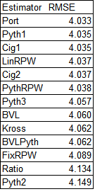
The RMSE shown here is actually the overall RMSE of the W% estimate, scaled to 162 games. So for each team the error is (W% - estimator)^2; the final value shown is 162*sqrt(average error):

Pythagenport has a slight lead over Pythagenpat, and they are followed very closely by the estimates based on Cigol and runs per win formulations that take RPG into consideration. In the Akousmatikoi family, that is the accuacy seperator (such that it is; the overall range of RMSE values is narrow) – considering the specific run environment for the team either through a Pythagorean approach (as in the case of Pythagenport, Pythagenpat, and their Cigol knockoffs), or a two operation (multiplication and addition) or power RPW function (as in the case of LinRPW and PythRPW). The next little cluster of RMSE includes a fixed Pythagorean exponent less than 2, the BenV-L formulas (which take the team’s RPG into account but only with a simple multiplicative function, not a y = mx + b form), and the intrepid Kross formulas. A fixed RPW linear approach is next, and then surpisingly, the Kross formuals actually outperform their antecedent (in the Akousmatikoi conceit, not reality) standard Pythagorean and “Ratio”, which uses a non-2 Pythagorean exponent.

This finding is surprising, and suggests that the Ratio approach should be discarded, as it’s arguably the most complicated to calculate of all the options we’ve looked at (despite being, at least from one perspective, a mathematical “simplification” of the Pythagorean relationship). But why does it perform worse than the Kross method, which ties to x = 2, while the ratio approach ties to x = 1.847, which has a lower RMSE than using x = 2?

To answer that question, I started by looking at the most extreme teams in terms of run ratio in the period, and found what I consider to be a satisfactory answer. The team with the highest run ratio in the expansion era is the 1969 Orioles (779/517 = 1.51). Incidentally, they do not have the highest Pythagenpat W% in the era, a distinction that goes to the 2001 Mariners by a hair’s breadth over the 1998 Yankees; those teams had run ratios of 1.48 and 1.47 respectively, but they had RPGs 20% and 25% higher respectively, which made their run ratios convert to higher win ratios.

The Orioles EW% using a fixed Pythagorean exponent of 1.847 is .681. This is the calculation that “Ratio” is supposed to flatten, but it predicts a W% of just .659. I think that since this formula is developed by differentiating win ratio, and then using the estimated win ratio to calculate an estimated W%,,the linear approximation does poorly. Win ratios have a much wider range than winning percentages; if we consider .300 - .700 a reasonably range for the expected (as oposed to actual) W%s of major league teams, this is a win ratio range of .429 to 2.333. Drawing the tangent line for the point where RR = WR = 1 leaves a lot of room outside of this range where teams will fall.

The Kross formula performs better because even though (in the Akousmatikoi sense) it starts from a less accurate proposition that x = 2, it will produce a wider range of win ratio estimates. The Kross estimated win ratio for a team with a run ratio of 1.51 is 2*1.51 – 1 = 2.02, while the other approach estimates 1.847*1.51 - .847 = 1.94.

The other RMSE comparison I want to make is to Pythagenpat. Again, I am not trying to say that Pythagenpat is the standard by which all win estimators should be judged. However, it (or something similar like Pythagenport) is the most accurate version of the Pythagorean relationship that has yet been published, and since this series is an examination of alternative win estimators mathematically related to Pythagorean methods, I think it is worthwhile to see which of these alternatives hew most closely to the starting point:

The fact that the lowest RMSE is for the first Cigol estimate tells us only what we can see by observing it – that it is essentially the same formula with added terms to attempt (perhaps in vain) to increase accuracy at the extremes (this formula sets the Pythagenpat exponent to .27348 + .00025*RPG + .00020*(R - RA)^2 rather than .282). That next in line are two more close cousins, Pythagenport and the other Cigol estimate, is comforting but also uninteresting.

You’ll notice that the ranking of estimators in terms of agreement with Pythagenpat closely resembles their ranking in accuracy predicting W%, so the first grouping of methods that most closely track Pythagenpat while actually being simpler to compute are the two RPW estimates that use a “complex” function – either the power relationship or the y = mx + b form.

The next cluster is an optimized fixed Pythagorean exponent and the Ben V-L approaches, which are equivalent to RPW as a multiplier of RPG (no y-intercept term). This implies that if you want to imitate Pythagenpat for normal teams, it’s most important to consider the impact of scoring level on the runs to wins conversion than it is to consider the non-linearity of the runs to wins conversion. The remarkable Kross formulas are next, with the others (a fixed RPW value, Pythagorean with x = 2, and the worthless “Ratio” approach) lagging the field.

I don’t have any grand conclusion to draw from this series, which is appropriate since as I’ve acknowledged previously, there really is nothing new here. It has served of a good reminder for me as to how various win estimators are connected, and hopefully has collected in one place observations of the connections that were previously published but strewn across multiple sources.

Trivia to close: I feel like I should have been aware of this previously, but did you know that (at least using a Pythagenpat z constant = .282), the 2019 Tigers had the worst EW% of the expansion era? They did not have the worst run ratio, a distinction that fell to the expansion 1969 Padres, but as we saw with the 1969 Orioles on the other end of the spectrum, the low RPG made that run ratio translate into a better win ratio than a couple of teams in higher scoring enviornments.

Four teams had sub-.310 EW%s (an arbitrarty cutoff as I think these four are interesting):

1. At .307, the expansion 1962 Mets, widely famous as the worst modern team and with the worst actual W% of the bunch at .250, are not a surprise.

2. At .305, the aforementioned 1969 Padres, a team I had never thought of as being historically bad for an expansion team. They actually went 52-110, a full twelve games better than the Mets, outplaying their Pythagenpat bytwo and a half games, whereas the ‘62 Mets underplayed theirs by nine. That explains it.

3. At .2998, the 2003 Tigers, who at 43-119 just missed matching the Mets record for most modern losses, although the Mets only played 160 games (40-120). This team is widely acknowledeged as one of the worst of all-time, but they underplayed their Pythagenpat by five and a half games.

4. At .2997, the 2019 Tigers, who only underplayed their Pythagenpat by one and a quarter games, going 47-114 and escaping historical notice. A big help was that they weren’t alone languishing at the bottom, as the phenomenon of “tanking” has been widely called out, and a number of teams over the last decade have put up truly terrible W-L records, including three others which lost 105 or more in 2019. The 2018 Orioles also served to take the heat off, as their 47-115 record was worse (they underplayed their Pythagenpat expectation by seven and a half games – they were only the thirteenth-worst of the expansion era at .337).