Simple BsR Component RAs

I suppose the adjective simple might be considered a misnomer by some readers; I'm referring more to the fact that all of the formulas in this post are going to be based on the same BsR formula. To get it out of the way upfront, I am at my core a lazy and hypocritical sabermetrician. I may write about the importance of sweating the small stuff, but when it comes down to it I pick one version of an equation and stick with it up until someone (occasionally even myself) demonstrates that it is flawed to the point of uselessness.

So I have a bit of an irrational attachment to this particular Base Run equation. It's not a horrible version, but it's not the best that one can come up with given these inputs either. I like it because the coefficients are easy to remember and it doesn't need to consider doubles and triples separately:

A = H + W - HR
B = (2*TB - H - 4*HR + .05*W)*x (approximately .78)
C = AB - H
D = HR
BsR = A*B/(B + C) + D

This formula will be used as the common starting point for a family of component RAs, each based on different inputs/approaches. I will run through four variants, three of which I have already used at some point on this blog. One commonality will be the use of run average as a unit rather than ERA. I have never cared for the distinction between earned and unearned runs and have always used RA. However, even if one does prefer ERA to RA, it still makes sense to express results in terms of total runs allowed. After all, the score is not kept in terms of earned runs. An equivalent RA is therefore much easier to work into other analytical methods, such as the Pythagorean formula.

As discussed in my previous post, there are a number of different logical paths to take in developing a component RA. The four that I use are the ones that I find most useful. None of them are unique to me--all of these constructions have been developed by others, and are simply being adapted here to specific categories and the BsR equation above. The point of this piece is to discuss the formulas and classify them, not to justify why I find them useful--as I said last time, that's a discussion that would require a separate post, one I don't feel like writing right now. The names I put on them are not intended to obscure that fact. The formulas all assume that one does not have actual opponent AB or PA; if you do, some of the estimation can be dispensed with.

I will be including all four estimators in my end of season stats next week, and giving them a separate post will reduce the clutter in the already wordy explanation that goes with the stats. 

1. Estimated Run Average (eRA)

eRA is the most straightforward flavor of component RA--a TRD estimator. There is very little manipulation of the BsR formula that goes into it:

A = H + W - HR
B = (2*TB - H - 4*HR + .05*W)*x (where x ~=.78)
C = AB - H = IP*y (where y ~= 2.82)
eRA = (A*B/(B+C) + HR)*9/IP

2. DIPS-style RA (dRA)

While the concept behind a DIPS RA has been well-known in sabermetrics thanks to Voros McCracken's work, it's still the most complex to calculate because one needs to reconstruct the pitching line, as innings pitched can no longer be treated as a constant. This is a TDD estimator.

Without using actual pitcher PA data, the first step is to estimate PA as IP*y + H + W (this estimate can be improved by spinning strikeouts off from innings, but I'm keeping it simple for this application). Then calculate the percentage of PA that result in walks, strikeouts, and home runs (I call these %W, %K, and %HR respectively). The percentage of balls in play (BIP%) is then just 1 - %W - %K - %HR. Multiplying BIP% by the league %H ((H-HR)/BIP) yields a new DIPS-estimate for %H.

Now everything is expressed as a rate with a common denominator of PA, and it's easy to plug in:

A = e%H + %W
B = (2*(z*e%H + 4*%HR) - e%H - 5*%HR + .05*%W)*x
C = 1 - e%H - %W - %HR
cRA = (A*B/(B + C) + %HR)/C*a

I've thrown in a couple more constants here; z is the league's average number of total bases per non-HR hit ((TB - 4*HR)/(H - HR)), generally around 1.28. a is the average number of AB-H per league game, generally around 25.2.

dRA is rate-based because it is easier to reconstruct the pitcher's line by just altering %H rather than constructing new estimates for hits and innings, which also change. There are equivalent approaches that would do just that.

3. Batted Ball class RA (cRA)

The obvious abbreviation here would be bRA--Dick Cramer used that once, but I'm going to pass. This is a TBD metric that considers batted ball types at their estimate values, without taking the SIERA route of giving line drives special treatment. tRA is the most famous metric that uses batted ball data in this way, but it uses linear weights and thus is classified as TBS. At least one other sabermetrician has already worked up a TBD metric of this type.

Admittedly, I am a little bit out of my element when working with the batted ball data. A metric like tRA is also a lot simpler than this one, because of the nature of using Base Runs. We cannot just take the linear weight for a groundball and calculate the needed BsR B weight to reproduce it for a given dataset, because we must be able to estimate baserunners, outs, and home runs from the batted ball types, rather than just needing the aggregate linear weight of the batted ball type.

This estimation, in my case at least, involves bringing in multiple sources of data--one which gives outcome (S, HR, etc.) frequencies for each batted ball type and another for the actual batted ball data for each pitcher. There are differences between data sources (STATS v. BIS v. Retrosheet) as well as other concerns about the uniformity of the data which makes this a significantly trickier task than estimating RA, and mean that formulas of this type will almost certainly need more upkeep over time.

Using the data from Colin Wyers here and the 2009 league totals of GB, FB, PU, and LD from Baseball Prospectus (here we have one of the data differences that I alluded to--Retrosheet v. BP's source) and reconciling to make sure that estimates of each hit type equals the actual 2009 totals, we get these equations:

cS = .057FB + .217GB + .516LD + .017PU
cD = .081FB + .018GB + .175LD + .004PU
cT = .0126FB + .001GB + .0155LD
cHR = .115FB + .024LD

We also need an estimate of outs, which I'll call cC because it plugs directly into the BsR equation:

cC = .6864FB + .7468GB + .2736LD + .9094PU + K

A = cS + cD + cT + W
B = (cS + 3*cD + 5*cT + 3*cHR + .05*W)*.742
cRA = (A*B/(B + cC) + cHR)*9/(cC*.3547)

4. SIERA-style RA (sRA)

SIERA is the new BP component ERA developed by Matt Swartz and Eric Seidman. I applied BsR in conjunction with what could loosely be described as a SIERA-style construction in this post, and so I won't go through each step again. Here I am presenting a different equation then in that post because this one is designed to estimate RA rather than ERA, but the logic is the same otherwise. Like cRA, this is a TBD metric--the difference is that batted balls are grouped in just two bins (grounders and non-grounders) rather than four:

nG = FB + LD + PU
G = GB
eS = .2167(G) + .2092(nG)
eD = .0184(G) + .1022(nG)
eT = .001(G) + .0119(nG)
eHR = .0701(nG)
A = eS + eD + eT + W
B = (eS + 3*eD + 5*eT + 3*eHR + .05*W)*.742
C = .76*G + .565*nG + K
sRA = (A*B/(B + C) + eHR)*9/(C*.355)

Poor Man's Pennant Race Standings (through 9/26/2010)

Relief Run Average

When it comes to picking the statistics I include in the spreadsheets I post here at the end of each season, my basic philosophy is to include only statistics that I can calculate myself (and that by extension the reader could calculate for himself) using data that is readily available. This necessarily results in using sub-optimal methods, as more advanced data (like that which can be culled from play-by-play accounts) can sharpen the focus of metrics and cut out some noise.

One example of this is in the adjustments I make to a pitcher's standard Run Average, a metric called Relief Run Average. The original RRA is based on Sky Andrecheck's article in the August 1999 By the Numbers, and uses inherited runner data to modify relief pitcher's RA. This year, using the data on bequeathed runners available at Baseball Prospectus, I've expanded RRA to consider both bequeathed and inherited runners for both starting and relief pitchers.

The major weakness of my approach is that I only consider the raw number of runners bequeathed and inherited (and their fates), not the base/out situation in which the pitching change is made. As such, it is not as comprehensive as the metrics available at BP which consider base/out state, and for pitchers with unusual patterns of bequeathed and inherited runners, the adjustments might actually make RRA a less accurate gauge of true performance than standard RA. On average, though, taking even the rudimentary data on runners into account will make for a more accurate evaluation of the pitcher, and so I use it.

Let me clearly define the statistical categories that go into RRA. IP and R are obvious, but we also have:

IR = inherited runners, IRS = inherited runners scored, BR = bequeathed runners, BRS = bequeathed runners scored, i = Lg(IRS/IR)

i is an important value that pops up twice in the formula. In the 2009 AL it was .337, while in the NL it was .303.

First, let's account for bequeathed runners. The number of bequeathed runners that can be expected to score is simply i*BR. We can compare this to BRS in order to get our crude estimate of bullpen support for the pitcher. The only issue is what positive and negative should indicate.

For inherited runners, I have always put a positive sign on "inherited runs saved" when the reliever performs better than expected. Since bequeathed runs saved will be the opposite of inherited runs saved, this suggests that the sign should be reversed. When the bullpen allows fewer bequeathed runners to score than expected, this means that the bequeathing pitcher's RA is lower than it otherwise would be.

A similar requirement is that if we add a pitcher's figures in the bequeathed and inherited categories, the signs should work out. Relievers will both bequeath and inherit runners, so they need to match up. Positive bequeathed runs saved (BRSV) offset positive inherited runs saved (IRSV). I realize that this explanation is confusing, perhaps it will be more clear when I run through an example for a reliever.

Let's start with a pitcher who made all of his appearances as a starter and thus had only bequeathed runners. Barry Zito is such a pitcher (33 appearances, all starts), and he led all exclusive starters with 27 bequeathed runners, of whom 11 scored. We would expect that 27*.303 = 8.18 would have scored, so Zito was charged with an additional 2.82 runs:

BRSV = BRS - BR*i = 11 - 27*.303 = 2.82

Zito was charged with 89 runs in 192 innings for a 4.17 RA. His RRA will be (89 - 2.82)*9/192 = 4.04.

Now let's look at a reliever who did not bequeath any runners. There are only four pitchers with 50+ innings in 2009 who did not bequeath a runner: three closers (Jenks, Papelbon, Valverde) and one remarkable starter (Halladay). Of the three relievers, Papelbon inherited the most runners (16, 4 of whom scored). We would have expected 16*.337 = 5.39 to score, so Papelbon saved an additional 1.39 runs:

IRSV = IR*i - IRS = 16*.337 - 4 = 1.39

Papelbon was charged with 15 runs in 68 innings for a 1.99 RA. His RRA is (15 - 1.39)*9/68 = 1.80.

Now let's consider the man who had the highest total of IR + BR, Grant Balfour. He bequeathed 43 of which 19 scored; we would have expected 14.49 to score, so his BRSV was 4.51, which means we're going to reduce his actual runs allowed by 4.51. On the other hand, he inherited 67 runners and allowed 18 to score; we would have expected him to allow 22.58, so his IRSV is 4.58. That means we reduce his runs allowed by a total (BRSV + IRSV) of 9.09 runs. He was charged with 38 runs in 67.1 IP for a 5.08 RA, but his RRA is figured using 28.91 runs and is thus 3.86.

These estimates will not always match with BP's Fair RA, which considers the actual base/out state. They have Balfour at 4.24, which is still a far cry from the standard 5.08 but also not as generous as RRA. If a relief pitcher tended to inherit runners in favorable base/out situations, then bequeath them without altering the base/out state too unfavorably, considering both bequeathed and inherited runners could overstate their effectiveness.

For example, suppose Balfour inherited all of his runners at first base with one out (obviously not a realistic example, but it makes the point), and faced only one righty in each case before being relieved for a left-hander. He would be inheriting runners in a favorable base/out state, then bequeathing them in an often more favorable state (if he recorded an out).

If you're going to account for inherited and bequeathed runners, it certainly is best to consider the base/out state as BP does. My contention with is simply that it is generally better to make the crude adjustment than no adjustment at all.

There's one important thing I haven't considered: park factors, which I overlooked in my previous applications of RRA as well. My old procedure was to add IRSV to runs allowed, then park adjust the entire RRA once constructed. However, this approach is flawed because it holds i constant across parks. Suppose a reliever in Coors Field allows 30.5% of his inherited runners to score. He will get negative IRSV. The park adjustment applied to his overall RRA will not change the fact that his RRA is higher than his standard RA, when in fact his performance in stranding inherited runners was likely above-average given the park.

So I've changed the way I apply the park factors this year. They are applied separately to each part of the RRA. I've assumed that the "i park factor" is equal to the square root of the standard runs park factor (PF). Square root adjustments are also good approximations for run components, and some very crude tests I ran suggest that it's a decent approach, at least one that is better than using PF with no adjustment or using the old, flawed method described above.

So the formulas are:

BRSV = BRS - BR*i*sqrt(PF)
IRSV = IR*i*sqrt(PF) - IRS
RRA = ((R - (BRSV + IRSV))*9/IP)/PF

I'll close with a couple of charts showing the largest percentage differences between RRA and RA in 2009. For these charts, no park factors were used and i was set equal to the 2009 major league average of .313 rather than a league-specific value.

First, the pitchers who take the biggest hit by using RRA:



All setup relievers, unsurprisingly. Saito and Howell can still be said to have pitched well when runners are taken into account, but the other three go from having adequate RAs to below-average (at least for a reliever).

The biggest beneficiaries:



Two closers and three setup men, all of whom appeared fairly effective through the lens of RA but were even more impressive when bequeathed and inherited runners are considered.

It is not surprising that RRA has the biggest effect on relief pitchers, who routinely bequeath and inherit runners. Starters never inherit runners, are more often pulled between innings, and appear in far less games. So here are the biggest moves for starting pitchers, limited to pitchers with more than 100 innings and no inherited runners for the season:



And the flip side:



AJ Burnett had a 4.30 RA, while his teammate Andy Pettitte allowed 4.67. However, the Yankees' pen allowed just one of Burnett's nineteen bequeathed runners to score, while fifteen of Pettitte's twenty-five scored. Pettitte accordingly bests Burnett in RRA, 4.34 to 4.52. Roy Oswalt had it worse--eleven of his twelve bequeathed runners came around to score.

Poor Man's Pennant Race Standings (through 9/19/2010)

Great Moments in Yahoo! Box Scores

For future reference: this was not an inside-the-park home run.

The Poor Man's Guide to the Pennant Race

There are a number of different statistical tools at one's disposal to aid in handicapping a pennant race based on the position of the teams at any given time. On the most basic level, we have games behind and magic number, two gauges that are understood by even the most stat-averse baseball fan. On the other side of the spectrum, there are several outlets that offer post-season probability estimates, of varying degrees of complexity and different inputs.

Suppose that you are caught somewhere between these two approaches; you are a sabermetrically aware fan who wants some indicators that you can figure with just the standings and a spreadsheet, eschewing the need for Monte Carlo simulation or a comparably complex tool. I have introduced (actually, rearranging more traditional approaches would be a better description) a few approaches on this blog over the last year or so. In this post, I'll summarize them and offer a quick look at the current standings.

What do these simple tools have in common other than not requiring advanced math to compute? The biggest thread is that because they keep it simple, they can only deal with comparisons between two teams, which makes them limited for races that include three or more teams. Another thing is that they rely on what I will call Game Outcomes Outstanding (GO). A game outcome is simply a win or a loss, but they include your opponent. For example, a team one game behind needs two positive game outcomes to move into first--a win for them and a loss for their opponent. Of course, if they are playing head-to-head, this could be accomplished in just one game, but for the purposes of this post, I still consider that to be two game outcomes. That's another thing the tools here have in common--they assume that teams never play head-to-head.

(1) The first tool is what I called "true GB", even though I didn't like the name. I'll change it to Effective GB here. Traditional games behind only considers a team's position relative to the division leader; it doesn't take into accounts the other non-leader teams that are in front of the team in question. To account for this, John Dewan proposed "GBsum", which sums up all of the deficits a team faces. If the Alphas trail the Bravos by 4 games and the Charlies by 3 games, their GBsum is 7.

I proposed Effective GB because GBsum would have us believe that being in the Alphas' position is just as bad as being seven games behind one opponent? But is that really true? On an fan's emotional level, I think most people would gladly choose to be in third place, four out of first and three out of second, then to be in second, seven games out.

I would argue that there is a simple and accurate explanation for this preference. The Alphas in theory could get into first place by winning four games, having the Bravos lose four and the Charlies lose three--eleven positive game outcomes. But in order to make up a seven-game deficit against one opponent, you need fourteen positive game outcomes--seven wins and seven opponent losses.

So Effective GB takes this into account by figuring the games behind the leader, which is the number of wins needed, and adding one-half of the games behind the other teams (which accounts for the opponent losses needed). The math works out so that:

Effective GB = (GB + GBsum)/2

An annoyance of Effective GB is that it's somewhat abstract--it can't be explained as easily in English as normal GB, and it offers up "quarter-games" (your Effective GB could be 3.25, for instance), which even for people used to the idea of "half-games" are tough to swallow.

(2) The second tool is the magic percentage (M%). M% is a close cousin to the magic number; it simply contextualizes it by dividing M# by the total number of games outstanding between the two teams. That means that the M% is the percentage of outstanding game outcomes that must go in the team's favor in order to win the title outright.

M# is a total; as with all totals, it ignores opportunities. There is a big difference between having a M# of 5 with two weeks to go in the season and having a M# of 5 with one weekend to go. In the first case, the pennant is all but secured; in the second, it's all but lost. Of course, M% as a rate leaves out important context as well. Everyone will start the season with their M% around .500; those that have a M% of around .500 by the end of the season are legitimate contenders. M% is not intended to replace M#--it is intended to complement it, just as batting average complements the raw hit total.

I already said it, but it bears repeating--M% is the proportion of favorable game outcomes outstanding that must go in a team's favor in order to win outright. For this reason, the M% of the two teams under consideration will not add to 1, since there is always a possibility of a tie. The fewer game outcomes are left outstanding, the further the sum of the two will diverge from 1. You could figure M% needed to ensure a tie as well by simply subtracting one from M# before calculating M%, but I'll stick with the M# construct of outcomes needed to win.

(3) The third tool is Crude Playoff Probability (CPP). CPP takes M# and GO, makes some simplifying assumptions (most importantly: no head-to-head games; all teams and opponents are true .500 teams; only two teams are in contention; the games outstanding are equally divided between both teams), and uses the binomial distribution to estimate the probability of winning the race (CPP does consider the possibility of a tie, and assumes a 50% chance of winning the resulting playoff game).

I wrote about CPP at length last week, so I won't rehash it again in detail. Instead, I'll reemphasize that CPP could also be called generic playoff probability. There is actually a finite number of possible games outstanding/games behind combinations, and one could produce an entire CPP table.

Here is just a small excerpt of such a table, showing the CPP from the trailing team's perspective for a number of GB/GO combinations (essentially every month throughout the season). In this case, games outstanding is from the perspective of one team only--the two teams are assumed to be on the same schedule (i.e. there are never any half-games in the standings). With this simplifying assumption, M# = GO (one team) - GB + 1. Remember that CPP only deals with the probability of catching one other team, not multiple teams.



This chart gets at the heart of why I designed (that is an extraordinarily haughty word choice of this situation, but I can't think of anything better) CPP. It certainly wasn't to improve on other people's published playoff odds, because CPP is quite obviously a step backwards. It was to address questions like "Would you rather be 5 games back with a month to play or 2 games back with a week to play"--questions which require a generic method when asked without a specific scenario in mind. Answer: the latter, 15.1% to 8.9%. What about five back after April or three back entering September? Assuming your team as good as the one it's chasing (which is an assumption that should be questioned if they are five back in one month), it's a toss-up: 27.2% to 29.5%. Given the limitations of CPP, none of this is intended to be authoritative, just food for thought.

Here are the standings through September 12, along with the poor man's indicators. Remember that M#, M%, and CPP for teams in third place or lower compare them only to the first place team, not to the teams in front of them; for the second place team, they relate to only the team they trail, not those behind them; and for the first place team, the only comparison is to their closest pursuer. GL is games left for the team in question; GO is total games outstanding for themselves and the first-place team (or the second-place team in the case of the first-place team):





Finally, to end on an only semi-related digression about something I surely have written about before, why does conventional wisdom say that it's better to be behind in the win column than behind in the loss column? Part of it is that being behind in the win column means that the difference can be made up by winning games that your team has yet to play, and so you "control your own destiny". From a probability perspective, though, that and a buck will get you a small fry.

The probabilistic reason why it's better to behind in the win column is that you'd rather have games outstanding than your opponent--assuming that you are both > .500 true quality teams. If the two teams in a pennant race are .550, you have a 55% chance of a favorable outcome when you play but only a 45% chance when your opponent plays.

The flip side of this is that if you have a race in which teams are < .500, you'd rather be ahead in the win column. Force the other team to go out and win games to catch you; don't try to do it yourself. No one really cares about races between bad teams, but it's something to keep in mind if you're checking the standings hoping to see your team avoid finishing in the cellar.

(Very) Crude Playoff Probabilities

If you are interested in what follows, then you will want to read my post on magic numbers and "magic percentage". That's the background material for this post.

In that post, I discuss the standard magic number, which is the number of game outcomes a team needs to go its way to clinch a playoff berth. I also introduced what I called magic percentage, which is the magic number divided by the total number of game outcomes outstanding--that is, games remaining for the team with the lead plus games remaining for the pursuer. The result is the percentage of favorable game outcomes needed to clinch.

As I pointed out, either form of the magic number leaves out some context. There's a big difference between having a magic number of one on the last day of the season and having a magic number of one with two weeks to play.

The magic percentage addresses that issue, but introduces its own. Two teams just about even in the standings will have M%s around .500, whether it is the first day of the season or the last.

As I said in the last post, if you really want to get serious, you can go the playoff odds route as implemented by Baseball Prospectus and others. Even then, there are a variety of different choices you can make about which factors to consider and how much complexity you are willing to tolerate.

Suppose we just want a crude estimate of playoff probability, and don't want to make any special assumptions about the two teams involved. Instead, we will assume the following:

* Only two teams are relevant in the race (obviously this is blatantly false early in the season, but is often true or close to true in September)

* The total number of outstanding games between the two teams is equally divided between the two (even if there is an odd number of total outstanding games and this is technically impossible)

* The outcomes of the games are independent--both for each team individually and the two collectively (so we're assuming that they're not playing each other)

* The two teams are of equal quality, and this quality is constant from game-to-game (so no home field advantage, and you are always playing against an average team)

After all of these caveats, you may be asking what the point of this exercise is. You are right to be asking that--as I've tried to make clear, I certainly am not asking you to stop considering sensibly constructed playoff probability estimates, or hoping to make you to eschew magic number for magic percentage or magic percentage for a crude probability. However, I personally do think that a crude playoff probability involving very few inputs is worth my time, and so I've shared it here.

What we're going to do is use the binomial distribution to estimate the probability of a team making the playoffs. Let's start with an easy case...there are four total outstanding games remaining, and the Alphas lead the Bravos by one game in the standings. Let's say they are 90-70 and 89-71 respectively. The Alphas have a magic number of two. That means that 2, 3, or 4 favorable game outcomes will result in a victory; 1 favorable outcome will result in a one game playoff; and zero favorable outcomes will give the Bravos the title.

What is the probability of a favorable outcome? Well, I've declared that the two teams are of equal quality, so it's close to 50%. Even if the two teams were true talent .900 teams, that would mean there is a 90% chance of a favorable outcome (for the Alphas) in an Alpha game and a 10% chance of a favorable outcome (for the Alphas) in a Bravo game.

Of course, this is a cheat--the weighted average of the individual probabilities does not capture the real dynamics of the situation, unless both teams are exactly .500. But for real teams, the discrepancies are not going to be as large, particularly over small numbers of games outstanding. If for instance you needed a .600 team to win and a .600 team to lose, the actual probability of that is .6*.4 = 24%; assuming that the probability is a uniform .5 results in an estimate of 25%. The differences could be greater over a longer period of games (*), so instead of saying that the probability of a favorable outcome is 50% as long as the two teams are of equal quality, it's safer to say that CPP assumes that all teams are of .500 true quality.

So, we can use the binomial distribution to figure the probability of X favorable game outcomes--there's a .5^4 = 6.25% that four outcomes go the Alphas' way, a (4 3)*.5^.3*.5 = 25% chance that three outcomes go their way, and a (4 2)*.5^2*.5^2 = 37.5% chance that two outcomes go their way, meaning the Alphas will win outright 68.75% of the time. There will be a one-game playoff (4 1)*.5*.5^3 = 25% of the time, which we expect them to win half of the time (12.5%), so the total probability of the Alphas winning the race is 81.25%.

To write this all up as a formula, let's christen this CPP for Crude Playoff Probability:

CPP = sum(n = M# to GO) [(n GO)*.5^n*.5^(GO - n)] + (M#-1 GO)*.5^(M# - 1)*.5^*(GO - (M# - 1))

If you want to plug this into Excel and take advantage of the cumulative binomial function, the formula is:

CPP = 1 - binomdist(M# - 1, GO, .5, true) + binomdist(M# - 1, GO, .5, false)/2

Where M# is the magic number and GO is the total games outstanding.

To rehash, CPP is the probability of winning a pennant race against another team assuming that:

1. teams are of constant quality from game-to-game, regardless of opponent or home field advantage
2. both teams are .500
3. game results are independent
4. there are no head-to-head games remaining between the two teams

That is a lot of qualifiers, which is why it is admittedly a crude probability.

Let's look at how CPP compares to M% for a team with a M# of two depending on how many game outcomes are outstanding:



Of course CPP approaches one much more quickly than the M% approaches zero, which is fine--the M% does not consider the exponential effect that slashes the probability of winning when you are coming from behind.

I also figured CPP for the MLB standings after games of September 24, 2009 (the day before I wrote this post). Here they are:



I really did this too late in the '09 season to be of any interest, as this year did not feature many close races and most of these were on the verge of being wrapped up. Still, it might be of interest to compare them to BP's estimate of the probabilities at the same moment. I looked at their normal postseason odds report; even though I definitely prefer the PECOTA-adjusted version, that one considers not just displayed team quality but the expected future performance of the players. The more layers of complexity that are added on, the less we expect the results to resemble those of CPP. Also keep in mind that CPP pretends as if there are only two teams involved in each race.

CPP gave the Red Sox a .6% chance to pass New York and the Twins a 9.5% chance to pass Detroit, while BP estimated 1.1% and 16% respectively. A large part of the difference is that the Red Sox and Yankees still had three games to play head-to-head and the Twins and Tigers had four. CPP gives the Rangers a .1% chance; BP said .2%.

In the NL, the two approaches agreed that the Braves had a .1% chance to win the division; BP held out .1% for the Cubs while CPP rounded it down to zero; and they agreed that the Rockies had a .2% chance to win the West. The wildcard race was the biggest difference; CPP had Colorado at 94.2% while BP gave them a 86.3% total playoff probability. The schedule had something to do with it, undoubtedly--seven of Colorado's's last ten games were against the Braves--as did the fact that San Francisco and Florida were still hanging around. However, CPP was much significantly less sanguine about Atlanta's hopes (5.8%) than was BP (9.9% to make the playoffs).

All in all, though, the correlation is pretty strong. The strength of CPP (simplicity) is also its weakness--it doesn't consider schedule, team quality, identity of personnel, home field advantage, etc. But the plus is that you save a lot of work and can fit the formula in Excel's formula bar. You would certainly want to be wary of CPP early in the season, as multiple teams are always in the hunt, but if at some point there is a clearly defined two-team race, it won't lead you too far astray, provided there aren't a very large percentage of head-to-head matchups remaining.

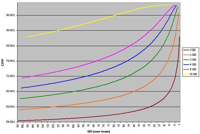
If we assume that both teams have played an equal number of games, then we can calculate M# as GO(one team) - GB + 1. Using this formula, here is a chart showing the CPP for a 1, 2, 3, 4, 5, and 10 game lead at each possible one-team GO value where a lead of that size to a) exist and b) have both teams still alive. So the line for a one game lead starts at 161 (games have to be played before a team can have a one game lead) and ends with 1 GO. The line for five games behind doesn't start until five games have been played (again, the earliest point at which a team can lead by five) and ends at five one-team GO (because any deeper into the season with a five game lead than that means the team has clinched):



In tribute to Bobby Thomson, here is a CPP chart for the Dodgers and Giants in 1951; remember that the probabilities relate only to the two rivals, not considering the other six NL clubs. I did not include the playoff series on the chart, because it would have produced a couple of wild swings which would detract from the picture of the race itself (New York won the first game and thus had a 75% probability, then Brooklyn won game two to bring it back down to 50%). The low point for Giant hopes was .3% on August 11, which is also the point of their largest deficit (13 games with 92 games outstanding).

The date that marked New York's true rise from the dead was September 25. Coming in, they trailed by two and a half with just eleven games outstanding, for a 7.3% CPP. The Giants beat the Phillies while the Braves swept the Dodgers in a doubleheader, leaving New York one back with eight outstanding for a 25.4% CPP. It was the first time their CPP had been in double digits since July 17, when they trailed Brooklyn by 7.5 with 137 outstanding (10.1% CPP), and the last time New York had been at a higher probability was July 3, when they were four back with 164 to play (26.7%).

Both teams won on the 26th, dropping Giants to 22.7%; on the 27th New York was idle while Brooklyn lost to Boston, leaving a half game margin with five outstanding (34.4%). Brooklyn lost to Philadelphia on the 28th to leave the teams in a tie with four outstanding, and both teams won their final two games to force the playoff, so the probabilities stayed at 50%.

Not including their 1-0 playoff lead, New York's highest CPP for the season was after Opening Day, when they established a one game lead on Brooklyn (54.5%). They dug an April hole (3-12, 23.7%), then won thirteen of eighteen to pull to within two games on May 19 (40%). June 2 (3.5 back with 223 games outstanding) marked their last time over 30% until late September (32%).



After the games of Sunday September 5, the CPPs for the race leaders against their respective second-place teams are:

NYA/TB: 75.6%
MIN/CHA: 83.4%
TEX/OAK: 99.3%
TB/CHA: 97.3%
ATL/PHI: 61.0%
CIN/STL: 97.1%
SD/SF: 60.8%
PHI/SF: 71.2%

I'll update this again in a week along with a rehashing of the easy gages of a team's position in the race.

(*) Suppose that over a period of 20 games (ten games each for two teams, no head-to-head games), we are interested in one of the team getting 15 favorable outcomes. CPP assumes that each game is a toss-up, and so the probability of 15/20 is just:

(20 15)*.5^15*.5^5 = 1.479%

Let's assume instead that the two teams are of equal true quality x. How many different ways can these 20 games combine for 15 favorable outcomes? We could have (10 wins, 5 losses), (9 wins, 6 losses), (8, 7), (7, 8), (6, 9), and (5, 10). The probability of (10, 5) can be broken down:

P(10 wins for Team A) = x^10
P(5 losses for Team B) = (10 5)*x^5*(1-x)^5
P(10, 5) = [x^10]*[(10 5)*x^5*(1-x)^5]

Repeating this calculation for all of the possible combinations that produce 15 favorable outcomes, here are the probabilities for several different values of x:



Assuming that both teams are .500 is in the ballpark for better teams, but far from a precise approximation. The accuracy of the approximation starts plummeting as one moves further away from .500, but that moves outside the range of true quality for major league teams. Even if there was such a team, it wouldn't be involved in a pennant race.

Perhaps I should have called it Generic Playoff Probability, because that's really what it is. Assume that it's a two-team race, and then pretend that all you know is the team's magic number and how many games are left to play.

Cory Luebke, #49

Cory Luebke made his major league debut for the Padres last night against the Rockies, becoming the 49th OSU major leaguer according to the Baseball-Reference list. (Incidentally, I was provided a list of possible OSU products via an unidentified late SABR member that numbers 58). In any event, Luebke joins Nick Swisher as the only active Buckeye major leaguer.

The last three OSU alums to make their debut include Luebke along with Josh Newman and Scott Lewis--all left-handed pitchers. Both Newman and Lewis are now out of major league baseball. Newman simply was not very effective and is now a newly-hired assistant coach for Greg Beals at OSU. Lewis pitched effectively for the Indians in 2008 and made the Opening Day rotation for 2009, but was injured in his home opening start against Toronto, never made it back up, and was released this spring after suffering another setback.

Hopefully Luebke is on the opposite of the Lewis career path, as his debut had its lumps. He went 5 innings, allowing 5 hits, 4 runs, 2 walks, 2 homers, 3 strikeouts, and throwing 46/78 pitches for strikes. He also took the loss for his now reeling team.

With Luebke now in the fold, it's natural to look for the next Buckeye prospect. Alex Wimmers was the Twins' first-round pick, and as a polished college pitcher he is obviously a candidate. Doug Deeds has had a good season in AAA for Arizona, but at 29 and without a spot on the 40-man roster he remains a long shot. Matt Angle has reached AAA in the Baltimore system, but he's an outfielder with limited power and hit just 259/333/303 this season. Jake Hale has been solid between two levels of A in the DBack system (47 K to 9 W in 43.1 IP), but he'll turn 25 in December and doesn't have dominant stuff. Eric Fryer, who caught at OSU but was moved to the outfield by the Yankees, has been moved back to catcher by the Pirates, exponentially increasing his chances. Unfortunately, he's 25 and has yet to make it out of A-ball, hitting 299/388/475 in 332 PA at A+ Bradenton. Other Buckeye minor leaguers have been hampered by drug suspensions (Ronnie Bourquin, Zach Hurley) , face a daunting combination of injury problems and advanced age (Dan DeLucia), or have a shot but were just drafted and are a long way away (Dan Burkhart).

The closest prospect is Houston's JB Shuck. A LHP/OF at OSU, JB now goes by "Jack" sometimes and is a full-time outfielder. He hit 298/372/360 at AA Corpus Christi and earned a promotion to AAA Round Rock, where in 143 PA he managed a 273/345/320 performance. As someone capable of playing CF in a thin system, Shuck is the best bet for a new Buckeye big leaguer in 2011.

At the time Lewis made his debut two years ago, RHP Mike Madsen seemed like the best bet, even being mentioned as a possible rotation candidate for Oakland, but he was done in by injuries.